I’m trying to learn more about Bayesian modeling, and I want to try to use Bugs/Jags/RStan. RStudio seems to have the most support for RStan (File -> New file has an option for a Stan file, but not the others). So my goal for now is to get a simple example working using RStan.
I started by following this blog post: https://www.r-bloggers.com/hierarchical-models-with-rstan-part-1/
Getting errors
Here’s the data in R that needs to be included.
#load libraries
library(rstan)
## Loading required package: ggplot2## Registered S3 methods overwritten by 'ggplot2':
## method from
## [.quosures rlang
## c.quosures rlang
## print.quosures rlang## Loading required package: StanHeaders## rstan (Version 2.18.2, GitRev: 2e1f913d3ca3)## For execution on a local, multicore CPU with excess RAM we recommend calling
## options(mc.cores = parallel::detectCores()).
## To avoid recompilation of unchanged Stan programs, we recommend calling
## rstan_options(auto_write = TRUE)## For improved execution time, we recommend calling
## Sys.setenv(LOCAL_CPPFLAGS = '-march=native')
## although this causes Stan to throw an error on a few processors.library(RColorBrewer)
#simulate some data
set.seed(20161110)
N<-100 #sample size
J<-10 #number of plant species
id<-rep(1:J,each=10) #index of plant species
K<-3 #number of regression coefficients
#population-level regression coefficient
gamma<-c(2,-1,3)
#standard deviation of the group-level coefficient
tau<-c(0.3,2,1)
#standard deviation of individual observations
sigma<-1
#group-level regression coefficients
beta<-mapply(function(g,t) rnorm(J,g,t),g=gamma,t=tau)
#the model matrix
X<-model.matrix(~x+y,data=data.frame(x=runif(N,-2,2),y=runif(N,-2,2)))
y<-vector(length = N)
for(n in 1:N){
#simulate response data
y[n]<-rnorm(1,X[n,]%*%beta[id[n],],sigma)
}rstan_options(auto_write = TRUE)Then I copied the Stan model into a file stan-test2.stan.
I used the second model with a non-centered parameterization.
Then when I tried to run it, I got an error.
#run the model
m_hier<-stan(file="./stan-test2.stan",data=list(N=N,J=J,K=K,id=id,X=X,y=y))
Error in compileCode(f, code, language = language, verbose = verbose) :
Compilation ERROR, function(s)/method(s) not created! Error in .shlib_internal(commandArgs(TRUE)) :
C++14 standard requested but CXX14 is not defined
Calls: <Anonymous> -> .shlib_internal
Execution halted
In addition: Warning messages:
1: In readLines(file, warn = TRUE) :
incomplete final line found on 'C:\Users\cbe117\Documents\GitHub\website-hugo\scratch\stan-test2.stan'
2: In system(cmd, intern = !verbose) :
running command 'C:/PROGRA~1/R/R-36~1.0/bin/x64/R CMD SHLIB file8403fc52d89.cpp 2> file8403fc52d89.cpp.err.txt' had status 1
Error in sink(type = "output") : invalid connectionAfter some Googling, I found a suggestion to add a line with
CXX14 = g++ -std=c++1y -Wno-unused-variable -Wno-unused-function -fPIC
into my Makevars.win file.
This removed the error, but I had another one.
#run the model
m_hier<-stan(file="./stan-test2.stan",data=list(N=N,J=J,K=K,id=id,X=X,y=y))
Error in compileCode(f, code, language = language, verbose = verbose) :
Compilation ERROR, function(s)/method(s) not created! file84038d44756.cpp:1:0: warning: -fPIC ignored for target (all code is position independent)
^
In file included from C:/Users/cbe117/Documents/R/win-library/3.6/BH/include/boost/random/detail/integer_log2.hpp:19:0,
from C:/Users/cbe117/Documents/R/win-library/3.6/BH/include/boost/random/detail/int_float_pair.hpp:26,
from C:/Users/cbe117/Documents/R/win-library/3.6/BH/include/boost/random/exponential_distribution.hpp:27,
from C:/Users/cbe117/Documents/R/win-library/3.6/BH/include/boost/random/gamma_distribution.hpp:25,
from C:/Users/cbe117/Documents/R/win-library/3.6/StanHeaders/include/stan/math/prim/mat/prob/dirichlet_rng.hpp:5,
from C:/Users/cbe117/Documents/R/win-library/3.6/StanHeaders/include/stan/math/prim/mat.hpp:276,
from C:/Users/cbe117/Documents/R/win-library/3.6/StanHeaders/include/stan/math/rev/mat.hpp:12,
Error in sink(type = "output") : invalid connectionI was able to fix this by following the suggestion from this StackOverflow answer
I added a line with CXX14 = "C:\Rtools\mingw_64\bin\g++.exe" to my Makevars.win file,
and then it ran fine.
Running the model
I had some errors with this next chunk of code initially.
When knitting the R markdown document, it would give an error
at the end saying that the path doesn’t exist.
I put a try around the line of code, and now it doesn’t give the error.
This is weird, but it works, so I’m not going to worry about it.
Now the model works and gives the following output.
try(m_hier <- stan(file="./../../content/post/stan-test2.stan",data=list(N=N,J=J,K=K,id=id,X=X,y=y)))##
## SAMPLING FOR MODEL 'stan-test2' NOW (CHAIN 1).
## Chain 1:
## Chain 1: Gradient evaluation took 0 seconds
## Chain 1: 1000 transitions using 10 leapfrog steps per transition would take 0 seconds.
## Chain 1: Adjust your expectations accordingly!
## Chain 1:
## Chain 1:
## Chain 1: Iteration: 1 / 2000 [ 0%] (Warmup)
## Chain 1: Iteration: 200 / 2000 [ 10%] (Warmup)
## Chain 1: Iteration: 400 / 2000 [ 20%] (Warmup)
## Chain 1: Iteration: 600 / 2000 [ 30%] (Warmup)
## Chain 1: Iteration: 800 / 2000 [ 40%] (Warmup)
## Chain 1: Iteration: 1000 / 2000 [ 50%] (Warmup)
## Chain 1: Iteration: 1001 / 2000 [ 50%] (Sampling)
## Chain 1: Iteration: 1200 / 2000 [ 60%] (Sampling)
## Chain 1: Iteration: 1400 / 2000 [ 70%] (Sampling)
## Chain 1: Iteration: 1600 / 2000 [ 80%] (Sampling)
## Chain 1: Iteration: 1800 / 2000 [ 90%] (Sampling)
## Chain 1: Iteration: 2000 / 2000 [100%] (Sampling)
## Chain 1:
## Chain 1: Elapsed Time: 1.563 seconds (Warm-up)
## Chain 1: 1.872 seconds (Sampling)
## Chain 1: 3.435 seconds (Total)
## Chain 1:
##
## SAMPLING FOR MODEL 'stan-test2' NOW (CHAIN 2).
## Chain 2:
## Chain 2: Gradient evaluation took 0 seconds
## Chain 2: 1000 transitions using 10 leapfrog steps per transition would take 0 seconds.
## Chain 2: Adjust your expectations accordingly!
## Chain 2:
## Chain 2:
## Chain 2: Iteration: 1 / 2000 [ 0%] (Warmup)
## Chain 2: Iteration: 200 / 2000 [ 10%] (Warmup)
## Chain 2: Iteration: 400 / 2000 [ 20%] (Warmup)
## Chain 2: Iteration: 600 / 2000 [ 30%] (Warmup)
## Chain 2: Iteration: 800 / 2000 [ 40%] (Warmup)
## Chain 2: Iteration: 1000 / 2000 [ 50%] (Warmup)
## Chain 2: Iteration: 1001 / 2000 [ 50%] (Sampling)
## Chain 2: Iteration: 1200 / 2000 [ 60%] (Sampling)
## Chain 2: Iteration: 1400 / 2000 [ 70%] (Sampling)
## Chain 2: Iteration: 1600 / 2000 [ 80%] (Sampling)
## Chain 2: Iteration: 1800 / 2000 [ 90%] (Sampling)
## Chain 2: Iteration: 2000 / 2000 [100%] (Sampling)
## Chain 2:
## Chain 2: Elapsed Time: 1.459 seconds (Warm-up)
## Chain 2: 1.63 seconds (Sampling)
## Chain 2: 3.089 seconds (Total)
## Chain 2:
##
## SAMPLING FOR MODEL 'stan-test2' NOW (CHAIN 3).
## Chain 3: Rejecting initial value:
## Chain 3: Error evaluating the log probability at the initial value.
## Chain 3: Exception: normal_lpdf: Scale parameter is -1.07263, but must be > 0! (in 'model252824de3e1b_stan_test2' at line 38)
##
## Chain 3: Rejecting initial value:
## Chain 3: Error evaluating the log probability at the initial value.
## Chain 3: Exception: normal_lpdf: Scale parameter is -1.55901, but must be > 0! (in 'model252824de3e1b_stan_test2' at line 38)
##
## Chain 3: Rejecting initial value:
## Chain 3: Error evaluating the log probability at the initial value.
## Chain 3: Exception: normal_lpdf: Scale parameter is -1.03044, but must be > 0! (in 'model252824de3e1b_stan_test2' at line 38)
##
## Chain 3:
## Chain 3: Gradient evaluation took 0 seconds
## Chain 3: 1000 transitions using 10 leapfrog steps per transition would take 0 seconds.
## Chain 3: Adjust your expectations accordingly!
## Chain 3:
## Chain 3:
## Chain 3: Iteration: 1 / 2000 [ 0%] (Warmup)
## Chain 3: Iteration: 200 / 2000 [ 10%] (Warmup)
## Chain 3: Iteration: 400 / 2000 [ 20%] (Warmup)
## Chain 3: Iteration: 600 / 2000 [ 30%] (Warmup)
## Chain 3: Iteration: 800 / 2000 [ 40%] (Warmup)
## Chain 3: Iteration: 1000 / 2000 [ 50%] (Warmup)
## Chain 3: Iteration: 1001 / 2000 [ 50%] (Sampling)
## Chain 3: Iteration: 1200 / 2000 [ 60%] (Sampling)
## Chain 3: Iteration: 1400 / 2000 [ 70%] (Sampling)
## Chain 3: Iteration: 1600 / 2000 [ 80%] (Sampling)
## Chain 3: Iteration: 1800 / 2000 [ 90%] (Sampling)
## Chain 3: Iteration: 2000 / 2000 [100%] (Sampling)
## Chain 3:
## Chain 3: Elapsed Time: 1.548 seconds (Warm-up)
## Chain 3: 1.238 seconds (Sampling)
## Chain 3: 2.786 seconds (Total)
## Chain 3:
##
## SAMPLING FOR MODEL 'stan-test2' NOW (CHAIN 4).
## Chain 4: Rejecting initial value:
## Chain 4: Error evaluating the log probability at the initial value.
## Chain 4: Exception: normal_lpdf: Scale parameter is -0.238897, but must be > 0! (in 'model252824de3e1b_stan_test2' at line 38)
##
## Chain 4:
## Chain 4: Gradient evaluation took 0 seconds
## Chain 4: 1000 transitions using 10 leapfrog steps per transition would take 0 seconds.
## Chain 4: Adjust your expectations accordingly!
## Chain 4:
## Chain 4:
## Chain 4: Iteration: 1 / 2000 [ 0%] (Warmup)
## Chain 4: Iteration: 200 / 2000 [ 10%] (Warmup)
## Chain 4: Iteration: 400 / 2000 [ 20%] (Warmup)
## Chain 4: Iteration: 600 / 2000 [ 30%] (Warmup)
## Chain 4: Iteration: 800 / 2000 [ 40%] (Warmup)
## Chain 4: Iteration: 1000 / 2000 [ 50%] (Warmup)
## Chain 4: Iteration: 1001 / 2000 [ 50%] (Sampling)
## Chain 4: Iteration: 1200 / 2000 [ 60%] (Sampling)
## Chain 4: Iteration: 1400 / 2000 [ 70%] (Sampling)
## Chain 4: Iteration: 1600 / 2000 [ 80%] (Sampling)
## Chain 4: Iteration: 1800 / 2000 [ 90%] (Sampling)
## Chain 4: Iteration: 2000 / 2000 [100%] (Sampling)
## Chain 4:
## Chain 4: Elapsed Time: 1.404 seconds (Warm-up)
## Chain 4: 1.238 seconds (Sampling)
## Chain 4: 2.642 seconds (Total)
## Chain 4:Then the following commands to look at the parameter results.
print(m_hier,pars=c("gamma","tau","sigma"))## Inference for Stan model: stan-test2.
## 4 chains, each with iter=2000; warmup=1000; thin=1;
## post-warmup draws per chain=1000, total post-warmup draws=4000.
##
## mean se_mean sd 2.5% 25% 50% 75% 97.5% n_eff Rhat
## gamma[1] 1.97 0.00 0.17 1.64 1.86 1.97 2.07 2.31 2919 1.00
## gamma[2] -0.13 0.03 0.78 -1.74 -0.60 -0.12 0.33 1.40 970 1.00
## gamma[3] 2.77 0.01 0.47 1.80 2.48 2.78 3.07 3.70 1297 1.00
## tau[1] 0.00 0.02 0.39 -0.68 -0.33 -0.01 0.31 0.69 317 1.01
## tau[2] -1.19 1.44 2.11 -3.71 -2.51 -2.04 -0.60 3.07 2 3.67
## tau[3] 0.02 1.03 1.50 -2.11 -1.36 0.03 1.38 2.31 2 3.88
## sigma 1.05 0.00 0.09 0.89 0.99 1.04 1.11 1.24 2734 1.00
##
## Samples were drawn using NUTS(diag_e) at Mon Jun 03 09:38:37 2019.
## For each parameter, n_eff is a crude measure of effective sample size,
## and Rhat is the potential scale reduction factor on split chains (at
## convergence, Rhat=1).mcmc_hier<-extract(m_hier)
str(mcmc_hier)## List of 6
## $ gamma : num [1:4000, 1:3] 2.01 1.88 1.91 1.98 1.86 ...
## ..- attr(*, "dimnames")=List of 2
## .. ..$ iterations: NULL
## .. ..$ : NULL
## $ tau : num [1:4000, 1:3] 0.374 0.0366 -0.1408 -0.2421 0.4946 ...
## ..- attr(*, "dimnames")=List of 2
## .. ..$ iterations: NULL
## .. ..$ : NULL
## $ beta_raw: num [1:4000, 1:10, 1:3] 0.446 1.25 -1.098 -1.064 0.98 ...
## ..- attr(*, "dimnames")=List of 3
## .. ..$ iterations: NULL
## .. ..$ : NULL
## .. ..$ : NULL
## $ sigma : num [1:4000(1d)] 0.926 0.97 0.927 1.052 0.867 ...
## ..- attr(*, "dimnames")=List of 1
## .. ..$ iterations: NULL
## $ beta : num [1:4000, 1:10, 1:3] 2.18 1.93 2.07 2.24 2.34 ...
## ..- attr(*, "dimnames")=List of 3
## .. ..$ iterations: NULL
## .. ..$ : NULL
## .. ..$ : NULL
## $ lp__ : num [1:4000(1d)] -70.8 -61.5 -62.3 -60.3 -63.4 ...
## ..- attr(*, "dimnames")=List of 1
## .. ..$ iterations: NULLAnd now some plots to visualize the results.
#plot average response to explanatory variables
X_new<-model.matrix(~x+y,data=data.frame(x=seq(-2,2,by=0.2),y=0))
#get predicted values for each MCMC sample
pred_x1<-apply(mcmc_hier$gamma,1,function(beta) X_new %*% beta)
#now get median and 95% credible intervals
pred_x1<-apply(pred_x1,1,quantile,probs=c(0.025,0.5,0.975))
#same stuff for the second explanatory variables
X_new<-model.matrix(~x+y,data=data.frame(x=0,y=seq(-2,2,by=0.2)))
pred_x2<-apply(mcmc_hier$gamma,1,function(beta) X_new %*% beta)
pred_x2<-apply(pred_x2,1,quantile,probs=c(0.025,0.5,0.975))
cols<-brewer.pal(10,"Set3")
par(mfrow=c(1,2),mar=c(4,4,0,1),oma=c(0,0,3,5))
plot(y~X[,2],pch=16,xlab="Temperature",ylab="Response variable",col=cols[id])
lines(seq(-2,2,by=0.2),pred_x1[1,],lty=2,col="red")
lines(seq(-2,2,by=0.2),pred_x1[2,],lty=1,lwd=3,col="blue")
lines(seq(-2,2,by=0.2),pred_x1[3,],lty=2,col="red")
plot(y~X[,3],pch=16,xlab="Nitrogen concentration",ylab="Response variable",col=cols[id])
lines(seq(-2,2,by=0.2),pred_x2[1,],lty=2,col="red")
lines(seq(-2,2,by=0.2),pred_x2[2,],lty=1,lwd=3,col="blue")
lines(seq(-2,2,by=0.2),pred_x2[3,],lty=2,col="red")
mtext(text = "Population-level response to the two\nexplanatory variables with 95% CrI",side = 3,line = 0,outer=TRUE)
legend(x=2.1,y=10,legend=paste("Gr",1:10),ncol = 1,col=cols,pch=16,bty="n",xpd=NA,title = "Group\nID")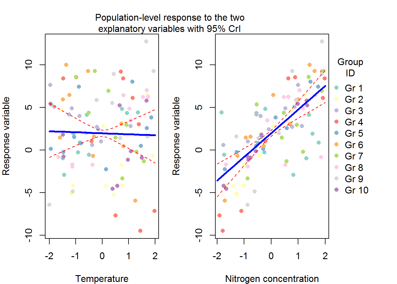
#now we could look at the variation in the regression coefficients between the groups doing caterpillar plots
ind_coeff<-apply(mcmc_hier$beta,c(2,3),quantile,probs=c(0.025,0.5,0.975))
df_ind_coeff<-data.frame(Coeff=rep(c("(Int)","X1","X2"),each=10),LI=c(ind_coeff[1,,1],ind_coeff[1,,2],ind_coeff[1,,3]),Median=c(ind_coeff[2,,1],ind_coeff[2,,2],ind_coeff[2,,3]),HI=c(ind_coeff[3,,1],ind_coeff[3,,2],ind_coeff[3,,3]))
gr<-paste("Gr",1:10)
df_ind_coeff$Group<-factor(gr,levels=gr)
#we may also add the population-level median estimate
pop_lvl<-data.frame(Coeff=c("(Int)","X1","X2"),Median=apply(mcmc_hier$gamma,2,quantile,probs=0.5))
ggplot(df_ind_coeff,aes(x=Group,y=Median))+geom_point()+
  geom_linerange(aes(ymin=LI,ymax=HI))+coord_flip()+
  facet_grid(.~Coeff)+
  geom_hline(data=pop_lvl,aes(yintercept=Median),color="blue",linetype="dashed")+
  labs(y="Regression parameters")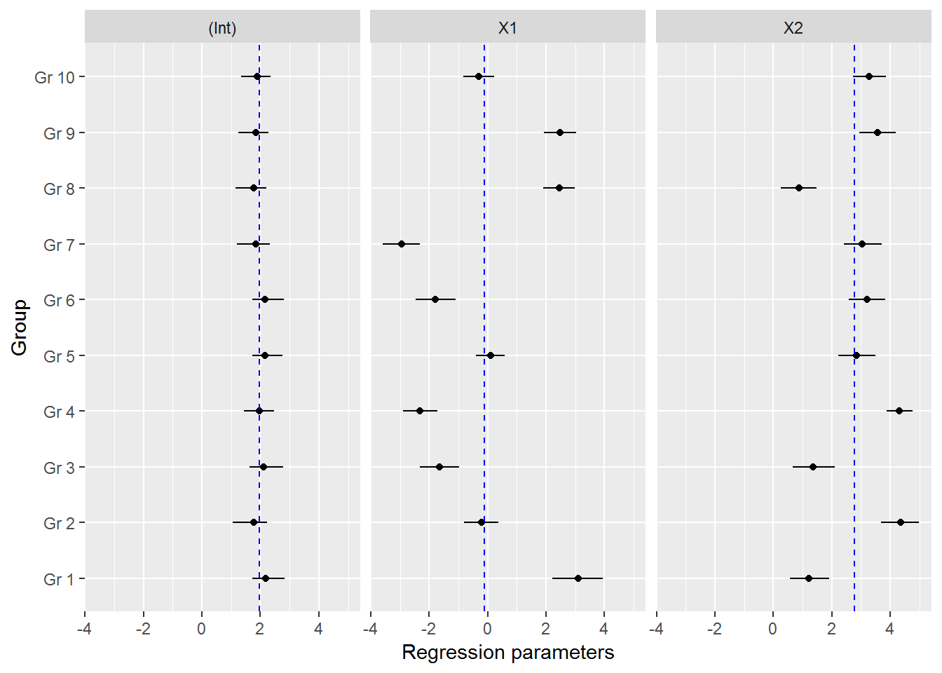
Conclusion
I used RStan for the first time and got it to work.
I just copy-pasted in an example.
As expected, I had some errors getting it to work on my computer.
I fixed them by adding a couple of lines to my Makevars.win file.
Another error weirdly disappeared by just putting the line in a try() call.
Now that I know RStan works on my computer,
I can begin actually editing the models and understanding the results.