Load packages
library(mlbgameday)
library(dplyr)
##
## Attaching package: 'dplyr'## The following objects are masked from 'package:stats':
##
## filter, lag## The following objects are masked from 'package:base':
##
## intersect, setdiff, setequal, unionlibrary(ggplot2)
library(magrittr)Get data. Using arbitrary dates.
dat <- get_payload(start = "2018-08-01", end = "2018-08-31")## Gathering Gameday data, please be patient...## Warning: executing %dopar% sequentially: no parallel backend registeredThis site is useful for deciphering fields.
dat$pitch has pitch data (location, speed, etc), dat$atbat has at bat data (result of at bat, etc),
so we need to join these.
# d2 <- inner_join(dat$pitch, dat$atbat, by=c("num", "url")) # All pitches are kept
# Keep only final pitches of each at bat
d2 <- inner_join(dat$pitch, dat$atbat, by=c("play_guid", "num", "url"))
event has the result of the atbat
d2$event %>% table %>% sort(decreasing = T)## .
## Strikeout Groundout Single
## 6873 5591 4690
## Flyout Walk Lineout
## 3496 2330 2001
## Pop Out Double Home Run
## 1596 1383 992
## Forceout Grounded Into DP Intent Walk
## 594 583 562
## Hit By Pitch Field Error Sac Fly
## 324 254 216
## Sac Bunt Triple Double Play
## 153 136 82
## Fielders Choice Out Bunt Groundout Runner Out
## 59 53 51
## Strikeout - DP Bunt Pop Out Fielders Choice
## 33 23 13
## Batter Interference Catcher Interference Fan interference
## 10 6 3
## Bunt Lineout Sac Fly DP Triple Play
## 2 1 1Let’s only keep the main events.
d3 <- d2 %>% filter(event %in% c("Strikeout", "Groundout", "Single", "Flyout", "Walk", "Lineout", "Pop Out", "Double", "Home Run"))There are 65 of these that don’t have px or pz. I’ll remove them.
d3$px %>% summary()## Min. 1st Qu. Median Mean 3rd Qu. Max. NA's
## -3.27056 -0.44091 0.02298 0.01852 0.47218 3.03732 65d3 <- d3 %>% filter(!is.na(px))Let’s look at where these occur in the strike zone.
ggplot(data=d3, mapping=aes(px, pz, color=event)) + geom_point(alpha=.2) + facet_wrap(. ~ event)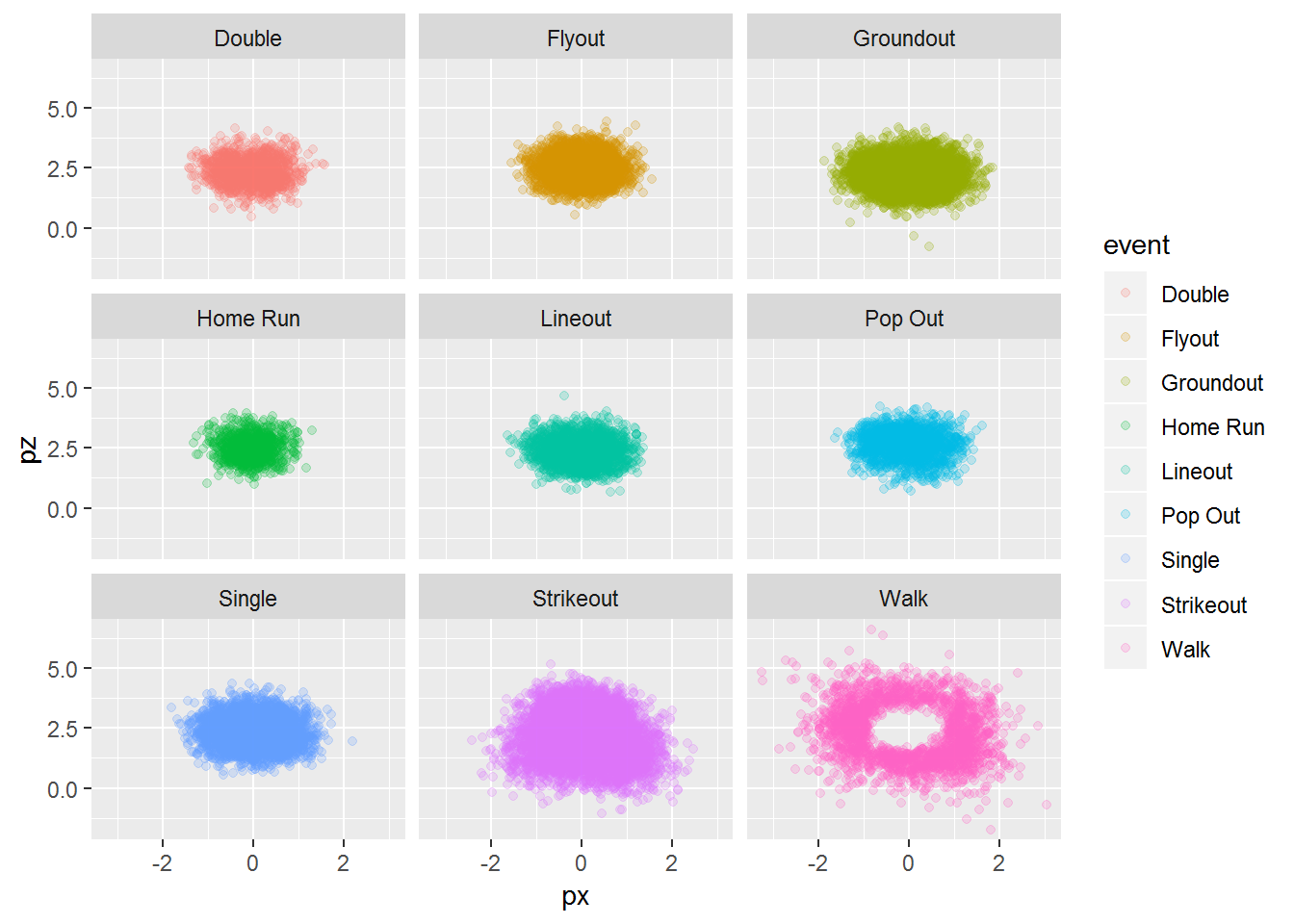
Unsurprisingly, walks are from out of the zone and extra base hits are in the zone.
ggplot(data=d3, mapping=aes(px, pz, color=event)) + geom_point(alpha=.2) + facet_wrap(. ~ event) + coord_fixed() + stat_density_2d()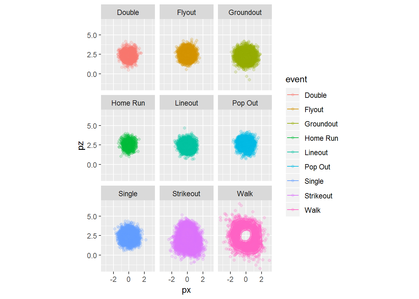
The zone will show which zone the pitched ended up in. 3x3 for the strike zone, four ball zones. These may change across batters (there is overlap comparing 3v4).
ggplot(data=d3, mapping=aes(px, pz, color=event)) + geom_point(alpha=.04) + facet_wrap(. ~ zone) + coord_fixed()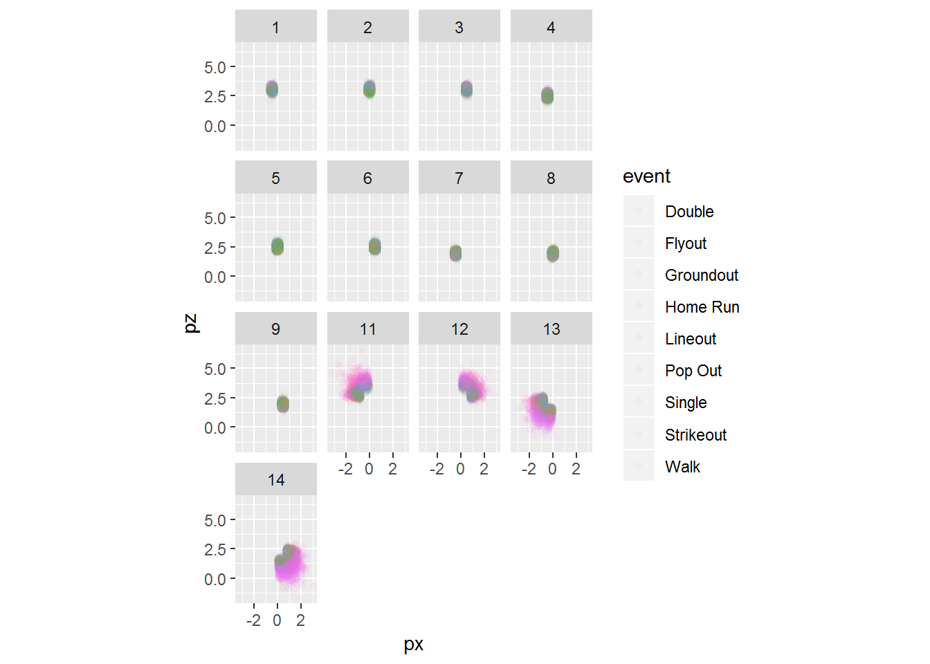
Here I’m making zones for the sake of plotting heat maps.
x <- c()
zone_values <- data.frame()
zones <- data.frame(
  zone = (c(rep(1:9, each=4), rep(11:14, each=6))),
  x = c(1,2,2,1,2,3,3,2,3,4,4,3,1,2,2,1,2,3,3,2,3,4,4,3,1,2,2,1,2,3,3,2,3,4,4,3,  0,1,1,2.5,2.5,0, 2.5,4,4,5,5,2.5, 2.5,5,5,4,4,2.5, 0,2.5,2.5,1,1,0),
  y = c(3,3,4,4,3,3,4,4,3,3,4,4,2,2,3,3,2,2,3,3,2,2,3,3,1,1,2,2,1,1,2,2,1,1,2,2,  2.5,2.5,4,4,5,5, 4,4,2.5,2.5,5,5, 0,0,2.5,2.5,1,1, 0,0,1,1,2.5,2.5)
)
zones$bs <- ifelse(as.numeric(zones$zone) <=9, "S","B")
ggplot() + geom_polygon(aes(x=x,y=y,fill=as.factor(bs), group=zone), zones, alpha=.5)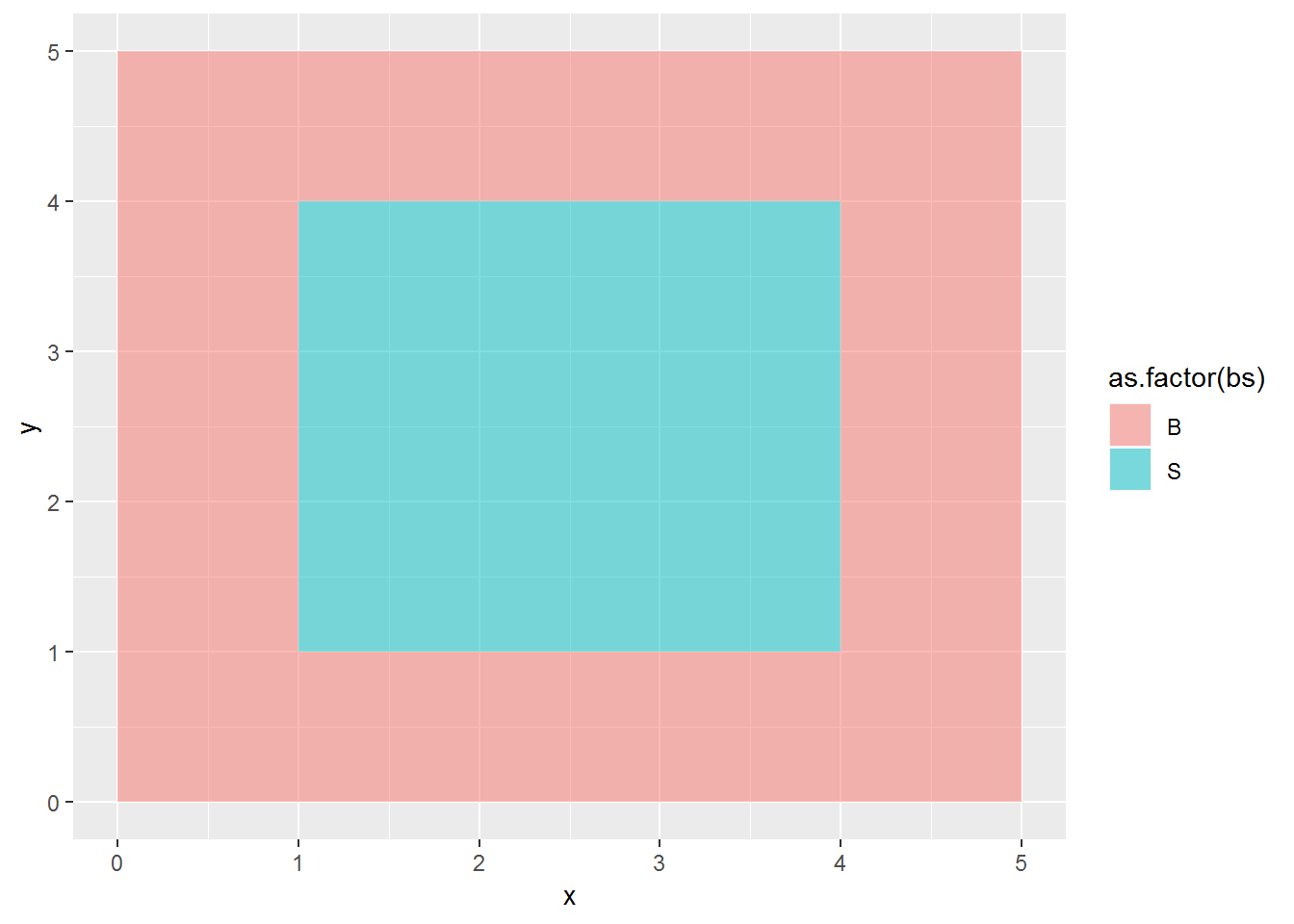
Okay, so now I want to show that for a given zone, what is the probability of it being a home run (or other event)?
First we’ll just group the events by their zone.
zone_events <- d3 %>% group_by(event, zone) %>% summarize(n=n())
zone_events %>% head
## # A tibble: 6 x 3
## # Groups: event [1]
## event zone n
## <chr> <dbl> <int>
## 1 Double 1 63
## 2 Double 2 60
## 3 Double 3 58
## 4 Double 4 160
## 5 Double 5 182
## 6 Double 6 128zone_events_total <- d3 %>% group_by(zone) %>% summarize(ntotal=n())
zone_events_total## # A tibble: 13 x 2
## zone ntotal
## <dbl> <int>
## 1 1 1139
## 2 2 1391
## 3 3 1158
## 4 4 2113
## 5 5 2476
## 6 6 2029
## 7 7 1680
## 8 8 2189
## 9 9 1901
## 10 11 2464
## 11 12 2008
## 12 13 3693
## 13 14 4646Now we join the zone_events with the total
zone_events2 <- dplyr::full_join(zone_events, zone_events_total, by="zone") %>% mutate(p=n/ntotal)
zone_events2 %>% head
## # A tibble: 6 x 5
## # Groups: event [1]
## event zone n ntotal p
## <chr> <dbl> <int> <int> <dbl>
## 1 Double 1 63 1139 0.0553
## 2 Double 2 60 1391 0.0431
## 3 Double 3 58 1158 0.0501
## 4 Double 4 160 2113 0.0757
## 5 Double 5 182 2476 0.0735
## 6 Double 6 128 2029 0.0631Now I’ll join with the zone locations.
zone_events3 <- full_join(zone_events2, zones, by="zone")
zone_events3 %>% head
## # A tibble: 6 x 8
## # Groups: event [1]
## event zone n ntotal p x y bs
## <chr> <dbl> <int> <int> <dbl> <dbl> <dbl> <chr>
## 1 Double 1 63 1139 0.0553 1 3 S
## 2 Double 1 63 1139 0.0553 2 3 S
## 3 Double 1 63 1139 0.0553 2 4 S
## 4 Double 1 63 1139 0.0553 1 4 S
## 5 Double 2 60 1391 0.0431 2 3 S
## 6 Double 2 60 1391 0.0431 3 3 SNow let’s try to plot it.
ggplot(zone_events3) + geom_polygon(aes(x=x,y=y,fill=p, group=zone), alpha=.8) + scale_fill_gradientn(colours=c('blue','white','red')) + facet_wrap(. ~ event)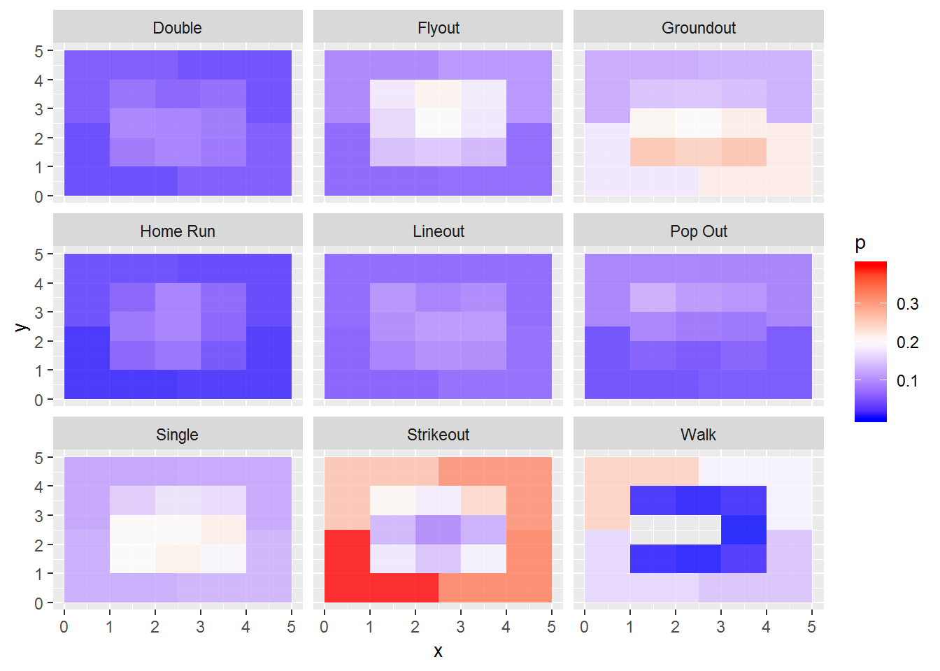
This plot looks reasonable. It says pitches in the bottom left lead to strikeouts. Pitches in the strike zone don’t lead to walks, and pitches in the strike zone don’t lead to walks. Groundouts result more often form pitches down than up.
It doesn’t look that good or useful. But it’s a start.