Looking at pitches with the R package mlbgameday

I’ll be continuing on from the last post.

Load packages first.

library(mlbgameday)
library(dplyr)

## 
## Attaching package: 'dplyr'

## The following objects are masked from 'package:stats':
## 
##     filter, lag

## The following objects are masked from 'package:base':
## 
##     intersect, setdiff, setequal, union

library(ggplot2)
library(magrittr)

Get some data.

dat <- get_payload(start = "2018-08-22", end = "2018-08-22")

## Gathering Gameday data, please be patient...

## Warning: executing %dopar% sequentially: no parallel backend registered

We’re going to be looking at dat$pitch.

dat$pitch %>% str

## 'data.frame':    4413 obs. of  50 variables:
##  $ des            : chr  "Ball" "Ball" "Called Strike" "Called Strike" ...
##  $ des_es         : chr  "Bola mala" "Bola mala" "Strike cantado" "Strike cantado" ...
##  $ id             : num  3 4 5 6 7 8 9 10 14 15 ...
##  $ type           : chr  "B" "B" "S" "S" ...
##  $ tfs            : chr  "163856" "163910" "163923" "163938" ...
##  $ tfs_zulu       : chr  "2018-08-22T16:38:56Z" "2018-08-22T16:39:10Z" "2018-08-22T16:39:23Z" "2018-08-22T16:39:38Z" ...
##  $ x              : num  80.4 62.1 93.8 79.4 83.4 ...
##  $ y              : num  175 154 162 174 166 ...
##  $ sv_id          : chr  "180822_163901" "180822_163915" "180822_163928" "180822_163942" ...
##  $ start_speed    : num  89.3 89.5 88.2 88.4 90 72.1 89.3 89.6 90 83.8 ...
##  $ end_speed      : num  79.8 79.7 79.1 79.4 81 65.5 79.7 81.1 81 75.8 ...
##  $ sz_top         : num  3.26 3.28 3.26 3.12 3.26 ...
##  $ sz_bot         : num  1.48 1.5 1.48 1.39 1.48 ...
##  $ pfx_x          : num  5.52 4.58 5.71 6.05 6.15 ...
##  $ pfx_z          : num  10.4 10 10.7 11.4 11 ...
##  $ px             : num  0.959 1.44 0.609 0.986 0.881 ...
##  $ pz             : num  2.37 3.15 2.83 2.4 2.7 ...
##  $ x0             : num  1.27 1.34 1.32 1.16 1.09 ...
##  $ y0             : num  50 50 50 50 50 ...
##  $ z0             : num  4.95 5.01 5.01 4.93 4.94 ...
##  $ vx0            : num  -2.62 -1.26 -3.66 -2.41 -2.59 ...
##  $ vy0            : num  -130 -130 -128 -129 -131 ...
##  $ vz0            : num  -3.67 -1.74 -2.59 -3.77 -3.17 ...
##  $ ax             : num  9.27 7.71 9.4 10.02 10.52 ...
##  $ ay             : num  31.4 32.2 29.7 29.5 31.3 ...
##  $ az             : chr  "-14.7786707194148" "-15.2884019002941" "-14.6331034350153" "-13.2149882308981" ...
##  $ break_y        : chr  "23.7" "23.7" "23.7" "23.7" ...
##  $ break_angle    : chr  "-28.9" "-25.2" "-29.4" "-34.0" ...
##  $ break_length   : num  4.3 4.2 4.3 4.2 4.1 15.1 4.7 4.6 4 8.8 ...
##  $ pitch_type     : chr  "FF" "FF" "FF" "FF" ...
##  $ type_confidence: num  2 2 2 2 2 2 2 2 2 2 ...
##  $ zone           : num  12 12 3 12 12 13 7 8 8 13 ...
##  $ nasty          : num  59 28 43 46 50 22 29 25 47 45 ...
##  $ spin_dir       : num  152 155 152 152 151 ...
##  $ spin_rate      : num  2202 2069 2251 2419 2397 ...
##  $ cc             : chr  "" "" "" "" ...
##  $ mt             : chr  "" "" "" "" ...
##  $ url            : chr  "http://gd2.mlb.com/components/game/mlb/year_2018/month_08/day_22/gid_2018_08_22_balmlb_tormlb_1/inning/inning_all.xml" "http://gd2.mlb.com/components/game/mlb/year_2018/month_08/day_22/gid_2018_08_22_balmlb_tormlb_1/inning/inning_all.xml" "http://gd2.mlb.com/components/game/mlb/year_2018/month_08/day_22/gid_2018_08_22_balmlb_tormlb_1/inning/inning_all.xml" "http://gd2.mlb.com/components/game/mlb/year_2018/month_08/day_22/gid_2018_08_22_balmlb_tormlb_1/inning/inning_all.xml" ...
##  $ inning_side    : chr  "top" "top" "top" "top" ...
##  $ inning         : num  1 1 1 1 1 1 1 1 1 1 ...
##  $ next_          : chr  "Y" "Y" "Y" "Y" ...
##  $ num            : num  1 1 1 1 1 1 1 1 2 2 ...
##  $ on_1b          : num  NA NA NA NA NA NA NA NA NA NA ...
##  $ on_2b          : num  NA NA NA NA NA NA NA NA NA NA ...
##  $ on_3b          : num  NA NA NA NA NA NA NA NA NA NA ...
##  $ count          : Factor w/ 12 levels "0-0","0-1","0-2",..: 1 4 7 8 9 9 12 12 1 2 ...
##  $ gameday_link   : chr  "gid_2018_08_22_balmlb_tormlb_1" "gid_2018_08_22_balmlb_tormlb_1" "gid_2018_08_22_balmlb_tormlb_1" "gid_2018_08_22_balmlb_tormlb_1" ...
##  $ code           : chr  "B" "B" "C" "C" ...
##  $ event_num      : chr  "3" "4" "5" "6" ...
##  $ play_guid      : chr  "6289c5d3-bcb1-4fbb-a972-b1f0ae888a19" "3c970495-dc61-4249-b36e-1b29f1bec006" "50cdbe92-3a4b-4c2d-b213-66e6406eee6b" "d0dc2bd6-31c2-4c85-8ad4-71c11cf2d517" ...

It looks like x and y are the coordinates where the pitch crosses the plate. And type is probably ball/strike.

ggplot(data=dat$pitch, mapping=aes(x, y, color=type)) + geom_point()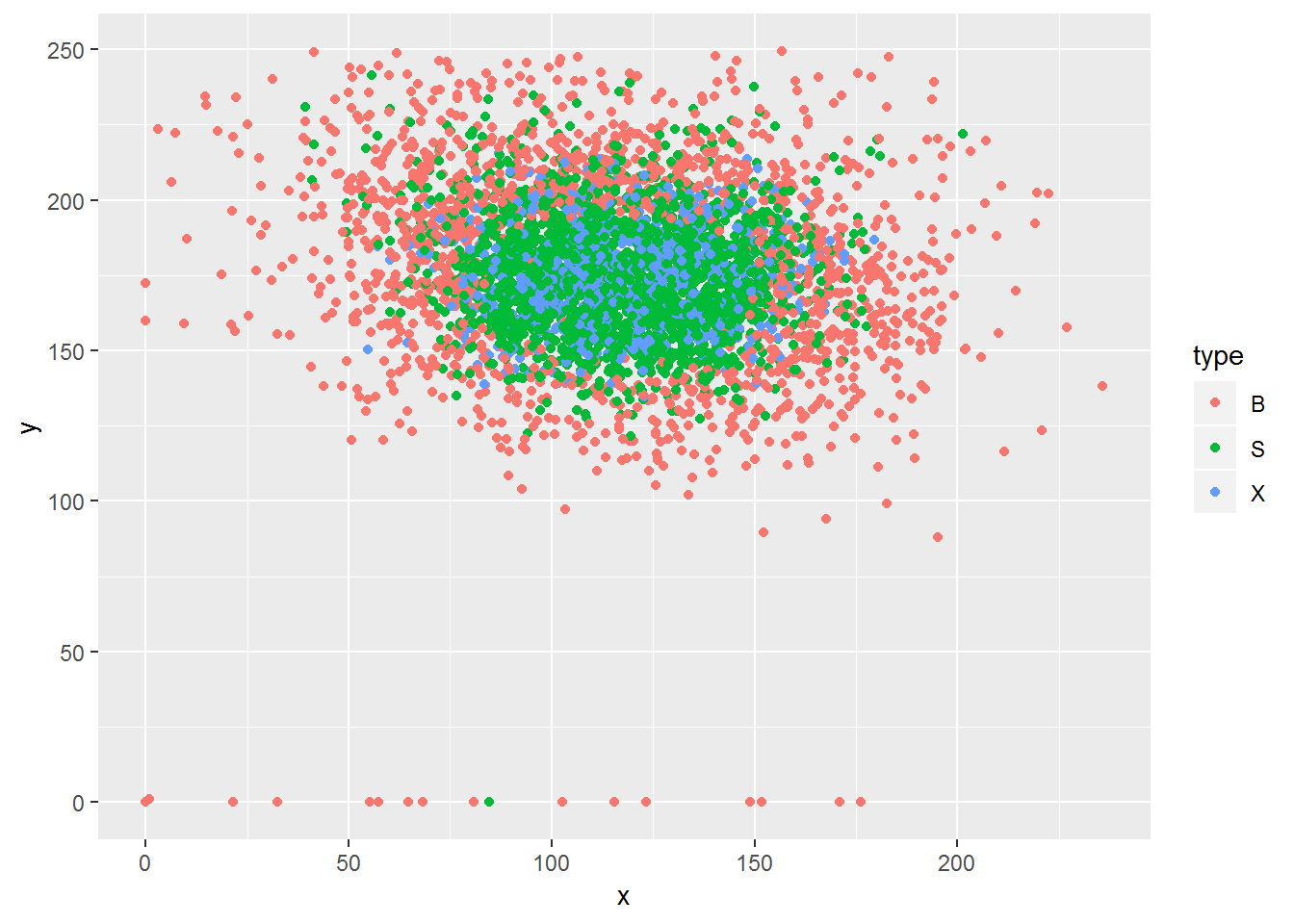

Let’s try faceting this into three plots.

ggplot(data=dat$pitch, mapping=aes(x, y, color=type)) + geom_point() +facet_grid(. ~ type)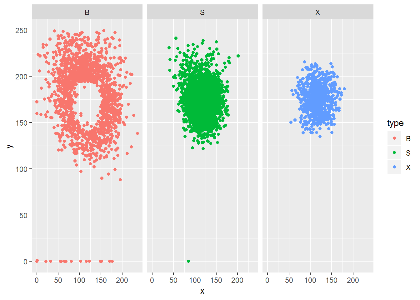

It looks like B is ball, but it’s not clear exactly what the difference is between S and X. Probably X is balls put in play, but does that include fouls? We’ll also want to separate out called strikes from swinging strikes. It looks like des gives a further distinction.

paste(dat$pitch$des, "///", dat$pitch$type) %>% table

## .
##            Automatic Ball /// B                      Ball /// B 
##                              16                            1468 
##              Ball In Dirt /// B             Called Strike /// S 
##                              91                             715 
##       Foul (Runner Going) /// S                      Foul /// S 
##                              13                             820 
##                 Foul Bunt /// S                  Foul Tip /// S 
##                              13                              33 
##              Hit By Pitch /// B           In play, no out /// X 
##                               9                             168 
##           In play, out(s) /// X           In play, run(s) /// X 
##                             508                             102 
##               Missed Bunt /// S                  Pitchout /// B 
##                               2                               1 
## Swinging Strike (Blocked) /// S           Swinging Strike /// S 
##                              36                             418

Indeed B is ball, but it also includes hit by pitch, pitchout, and automatic ball (not sure what that is). S includes strikes and fouls. X exclusively indicates balls put in play.

I’m going to filter out some of these des values that don’t occur very often using functions from dplyr.

pdf <- dat$pitch %>% group_by(des) %>% filter(n() > 100) %>% ungroup

ggplot(data=pdf, mapping=aes(x, y, color=des)) + geom_point()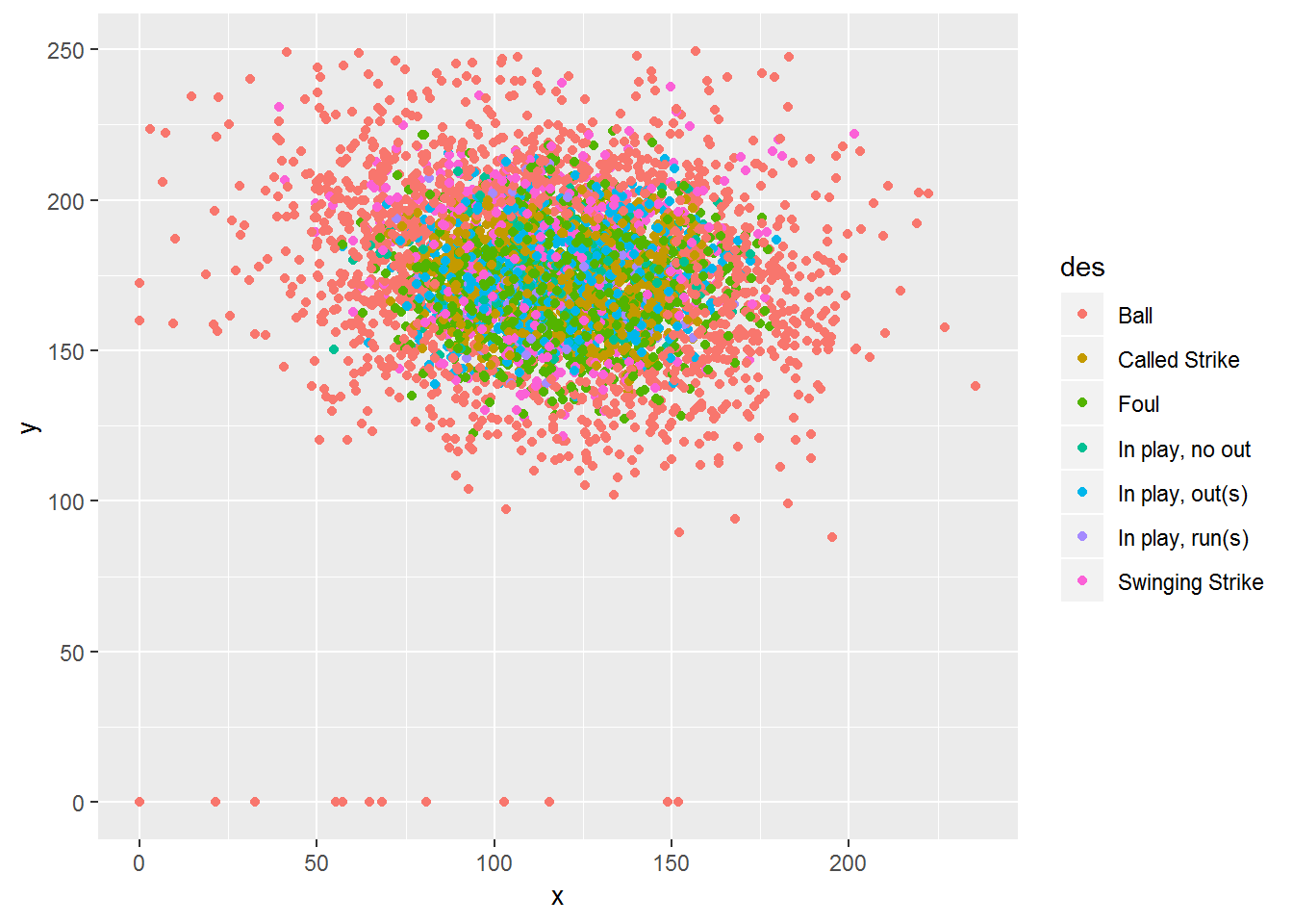

ggplot(data=pdf, mapping=aes(x, y, color=des)) + geom_point() + facet_wrap(. ~ des)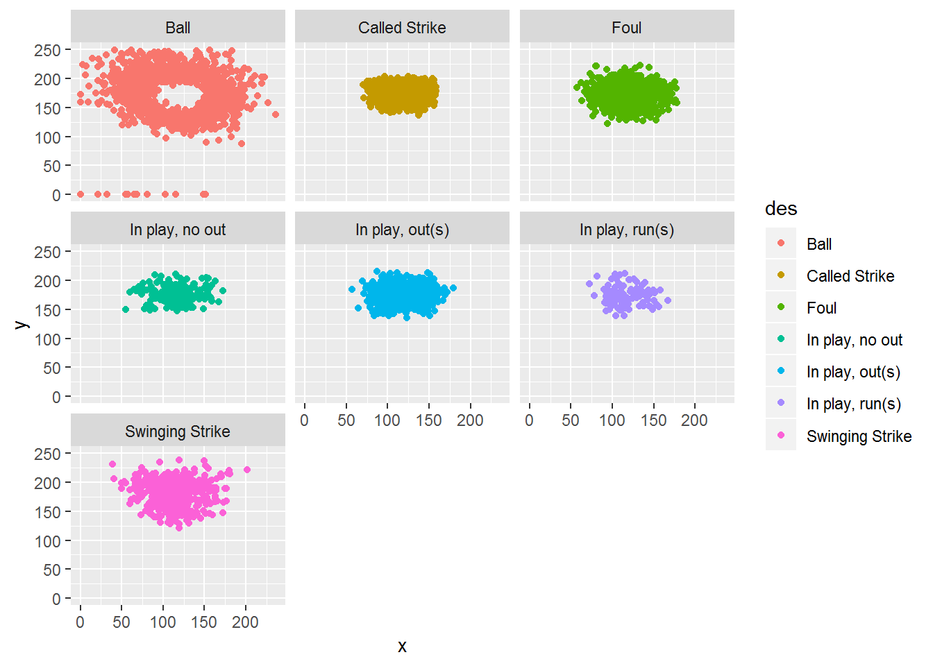

Nothing too surprising here. Now we can see that the division between Ball and Called Strike can be used to estimate the strike zone. I’m going to filter so only those two are left.

pdf2 <- (pdf %>% filter(des=="Ball" | des=="Called Strike"))

ggplot(data=pdf2, mapping=aes(x, y, color=des)) + geom_point(alpha=.25) + facet_wrap(. ~ des)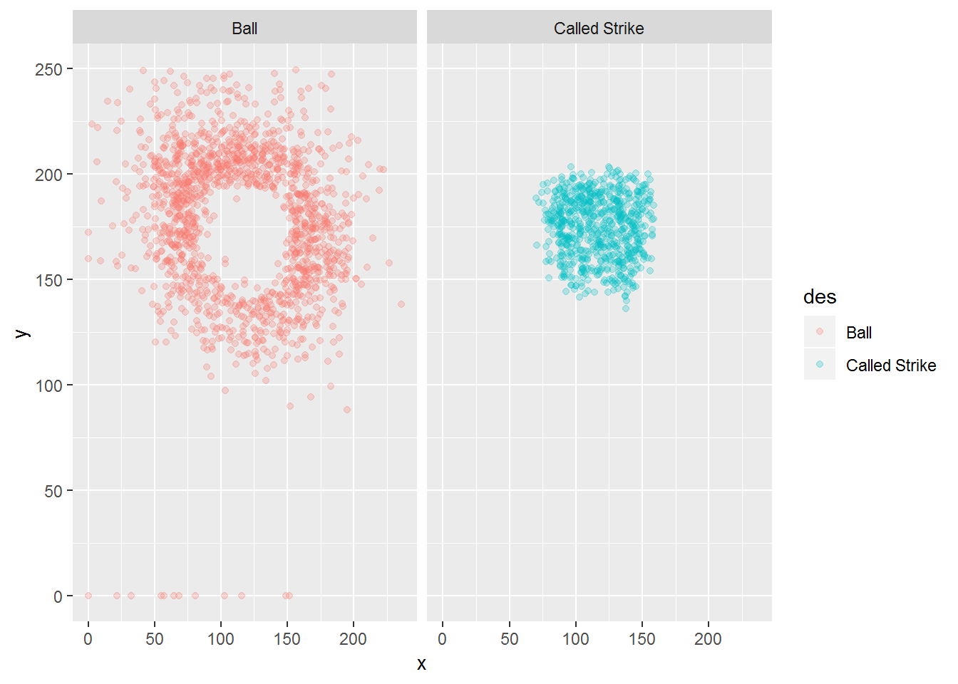

Using machine learning to classify balls and strikes

Now we can use this data to create a model that will be able to predict balls and strikes.

I’ll create a grid of data points that we can predict on and plot.

testdf <- expand.grid(x=seq.int(50,200,1), y=seq.int(100,250,1))

k nearest neighbors

The first method I’ll try is k nearest neighbors since it seems like it should work easily and it’s easy to understand. To predict whether a given pitch is a ball or strike, we simply find the k nearest neighbors (shortest distance from the point), and assign it the class that is the majority of the classes of those k points.

First we’ll use $k=1$.

knn1pred <- rep(NA, nrow(testdf))
apply(testdf, 1, 
      function(rowi) {
        print(rowi)
        dists <- sapply(1:nrow(pdf2), function(gi) {sum((rowi - pdf2[gi,c('x','y')])^2)})
        inc <- which.min(dists)[1]
        pdf2$des[inc]
      }
)

This is way too slow, and probably not even correct. I had to kill it because it would take all day to finish. I tried to do a simple implementation, but it is not efficient enough.

It’s always better to try to use an already existing package that has been optimized for performance. In this case we can use the R package class, and it’s function knn.

knn1_pred <- class::knn(train = pdf2[,c('x','y')], test = testdf, k = 1, pdf2$des)

Now let’s plot it and look at the classifications

knn1_pred2 <- data.frame(x=testdf$x,
                  y=testdf$y,
                  class=knn1_pred)
ggplot(data=knn1_pred2, mapping=aes(x, y, color=class)) + geom_point() + facet_grid(. ~ class)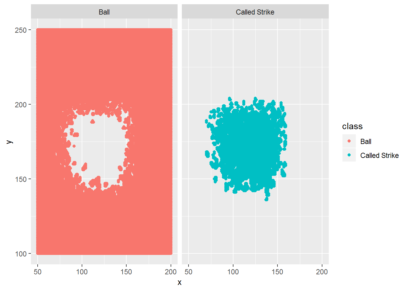

This looks reasonable based on the data we have. It not very smooth at the edges. We can try using a larger value for $k$. This will help smooth it out, but we need to be careful that it doesn’t get smoothed too much. Let’s try using $k=11$.

knn11_pred <- class::knn(train = pdf2[,c('x','y')], test = testdf, k = 11, pdf2$des)

knn11_pred2 <- data.frame(x=testdf$x,
                  y=testdf$y,
                  class=knn11_pred)
ggplot(data=knn11_pred2, mapping=aes(x, y, color=class)) + geom_point() + facet_grid(. ~ class)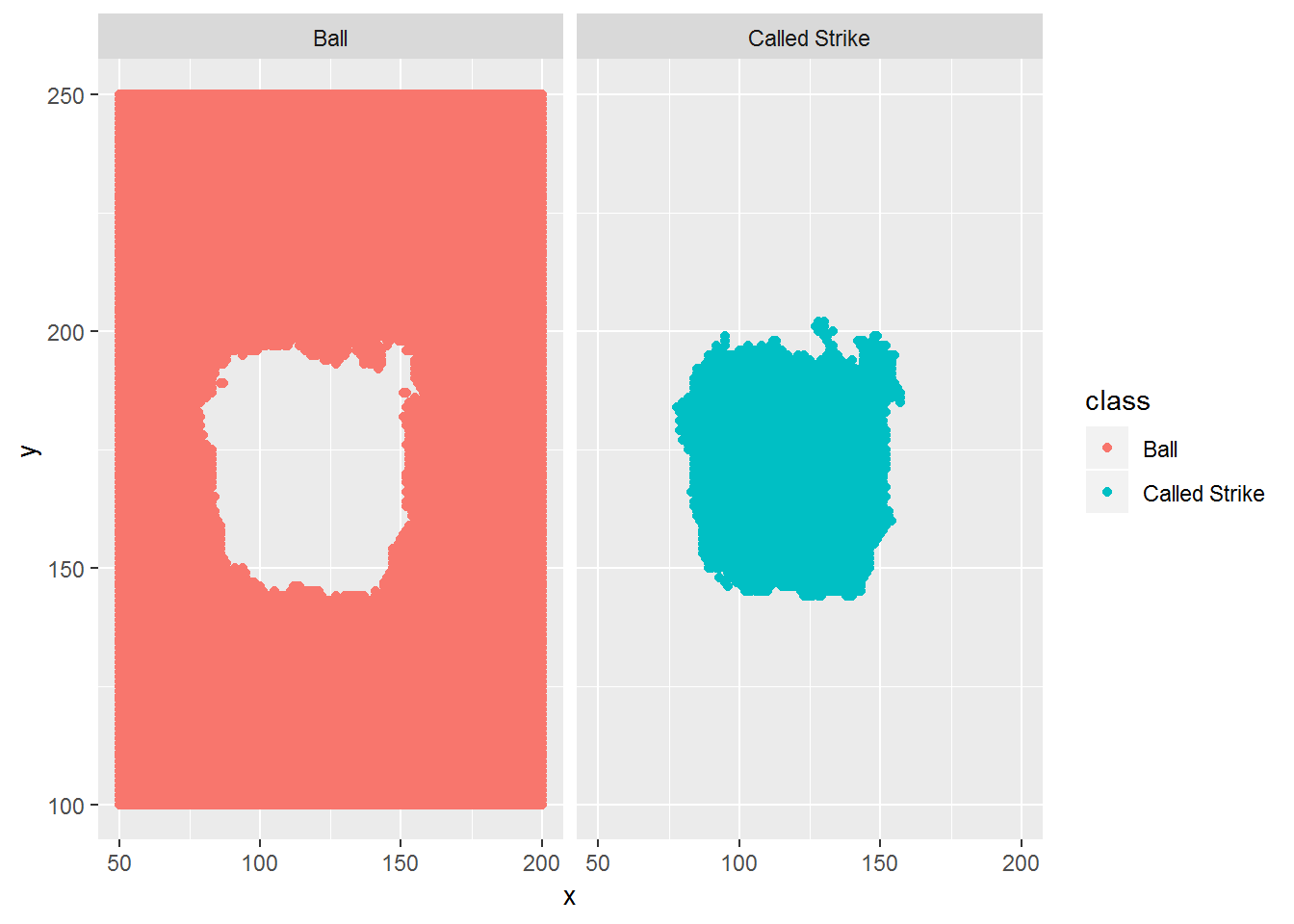

It is definitely smoother. We might hope for a perfect rectangle, but that would be unrealistic because umpires don’t make perfect calls, and we are limited by the data that we have.

Random forest

rf_pred <- randomForest::randomForest(x = as.matrix(pdf2[,c('x','y')]), xtest = as.matrix(testdf), y=as.factor(pdf2$des))

Now let’s plot it and look at the classifications

rf_pred <- data.frame(x=testdf$x,
                  y=testdf$y,
                  class=rf_pred$test$predicted)
ggplot(data=rf_pred, mapping=aes(x, y, color=class)) + geom_point() + facet_grid(. ~ class)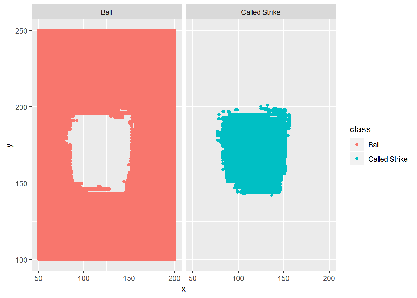

Again, this looks reasonable.

Conclusion

We’ve taken MLB data and created a model that can predict whether a given pitch should be classified as a ball or strike based on its coordinates when it crossed the plate.

With more data, we can look into how the strike zone changes based on the handedness of the batter, the type of pitch, and the count.