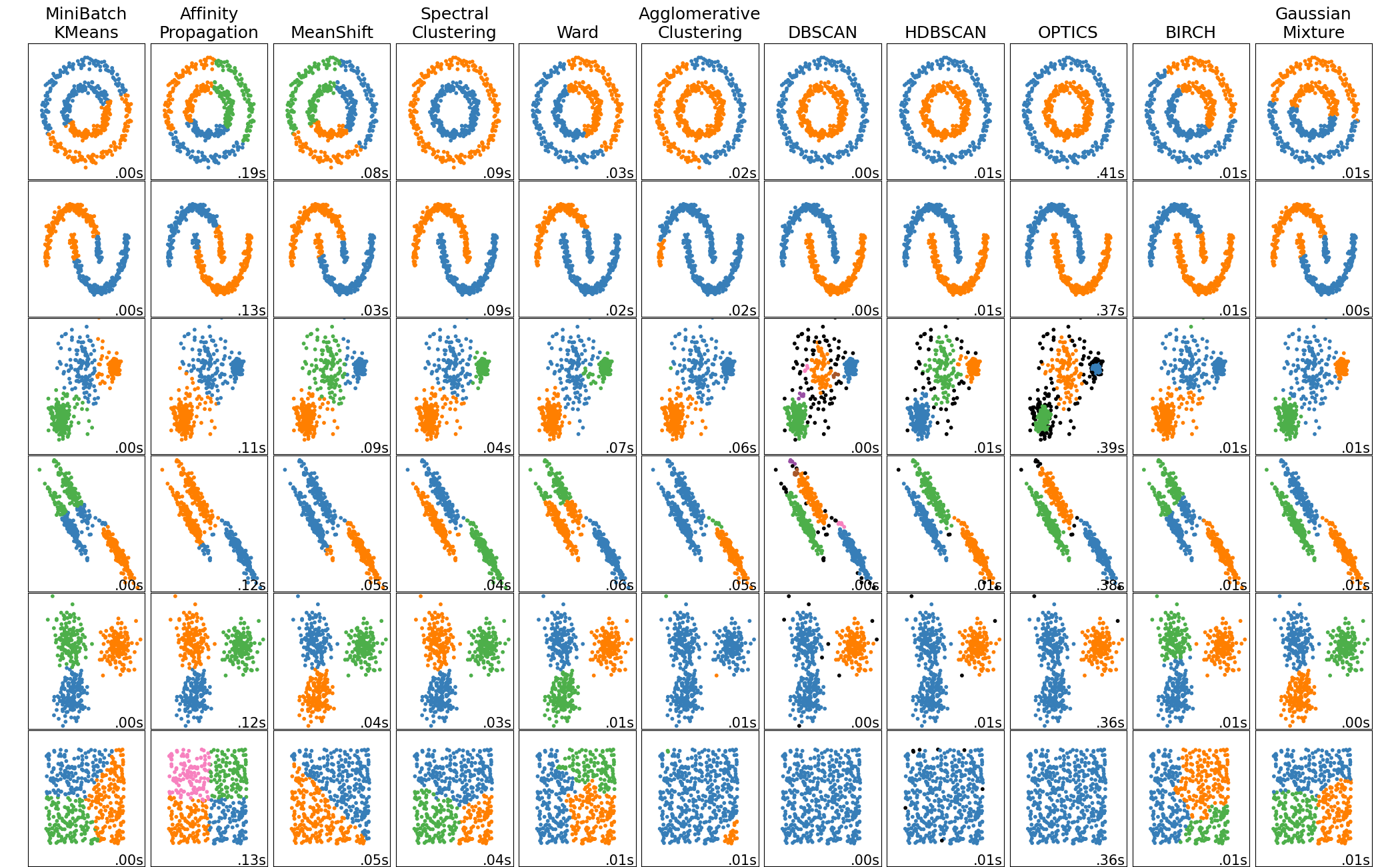
I had never heard of spectral clustering until last week. Then I came across this image comparing 9 clustering algorithms on different 2D datasets.
knitr::include_graphics("https://scikit-learn.org/stable/_images/sphx_glr_plot_cluster_comparison_001.png")
It appeared to me that spectral clustering did the best across all the data, and I realized that the only clustering algorithm I understood was k-means. (DBSCAN might be better based on the results shown, but one step at a time.) So here I’m going to try to figure out what spectral clustering is and how I can implement it.
How does it work?
Create data
I’m going to create a dataset to have something to work with as I go. I’m going to make it very easy to start with.
set.seed(0)
n <- 20
x1 <- matrix(rnorm(2*n), n, 2)
x2 <- sweep(matrix(rnorm(2*n), n, 2), 2, c(-15,0))
x <- rbind(cbind(x1,1), cbind(x2, 2))
x <- data.frame(x)
x[,3] <- as.factor(x[,3])
names(x)[3] <- "group"
library(ggplot2)
ggplot(data=x, mapping=aes(x=X1, y=X2, color=group)) + geom_point()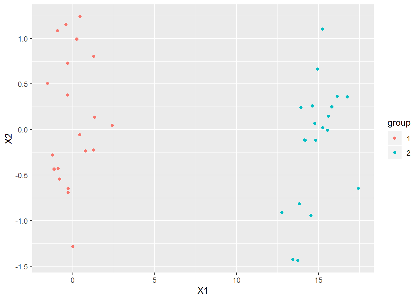
It’s obvious to tell what the two groups are by looking at the plot. Any clustering algorithm that got this wrong would be worthless.
Similarity matrix
First we have to create the similarity matrix. We can use a Gaussian measure to determine the similarity. There are many other ways this can be done, such as putting 1’s for the nearest neighbors, and 0 elsewhere.
S <- outer(1:(2*n), 1:(2*n), Vectorize(function(i,j, sig=3) {exp(-sum((x[i,1:2]-x[j,1:2])^2)/2/sig^2)}))Here’s what the similarity matrix looks like.
image(S)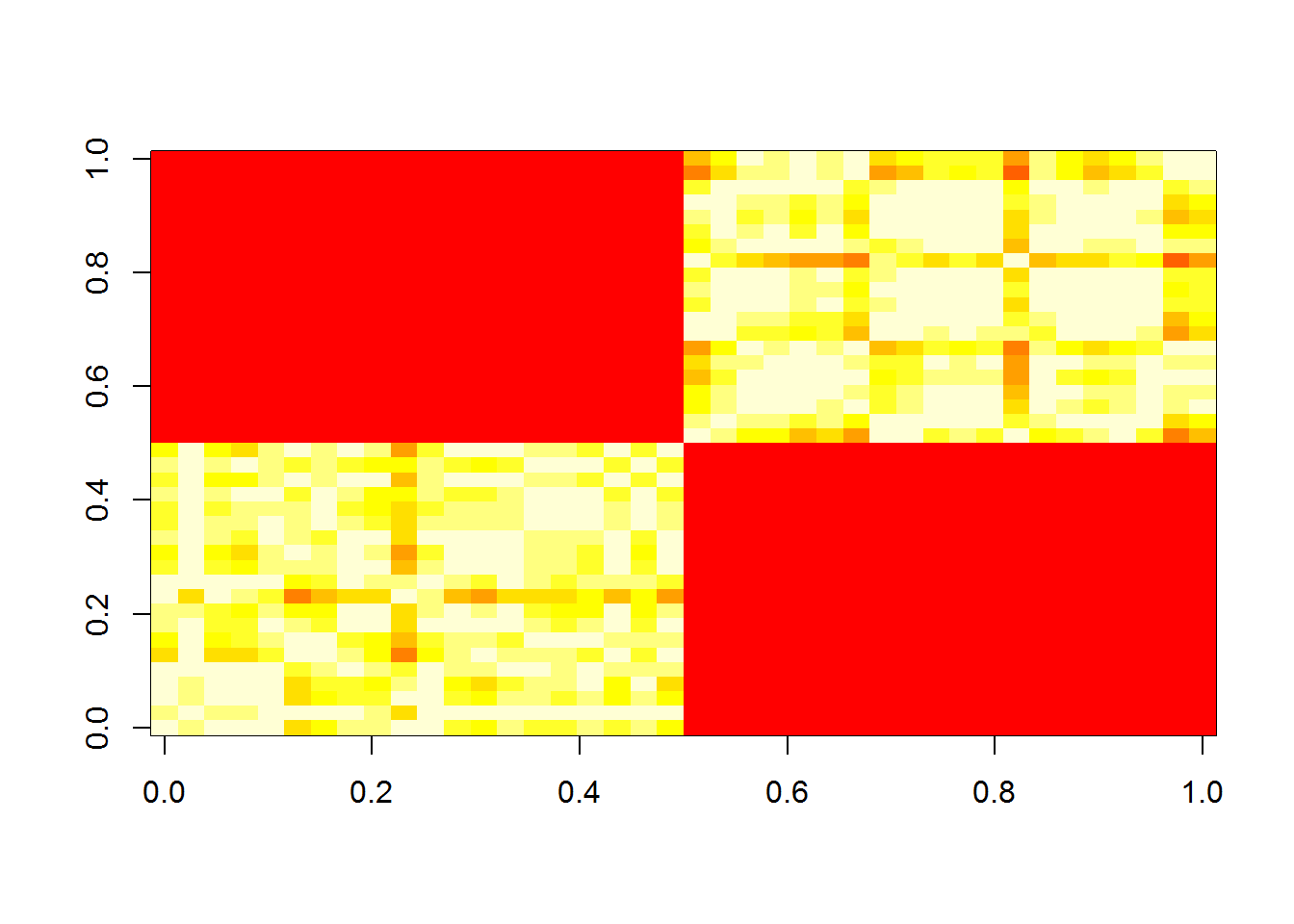
Weighted adjacency matrix
Next we need a weighted adjacency matrix to determine which points are close to each other. There are a couple of different ways to create this matrix.
We can use the similarity matrix as our weighted adjacency matrix since we are using the Gaussian for similarity.
W <- SDegree matrix
The degree matrix \(D\) is the diagonal matrix with the sum of the adjacent weights for each node.
D <- diag(rowSums(S))Laplacian matrix
Now the Laplacian matrix is \(L=D-W\).
L <- D - WEigenvectors
Now we calculate the eigenvectors of \(L\). \(U\) is the matrix with the eigenvectors as its columns.
# (L %*% eigen(L)$vec[,1] ) / eigen(L)$vec[,1]
U <- eigen(L)$vec
Here’s the key part. We take the \(k\) eigenvectors for the smallest eigenvalues.
k <- 2
N <- 2*n
Uk <- U[,(N-k+1):N]
k-means
Now we run k-means clustering on the rows of that matrix.
km.out <- kmeans(Uk, k)
library(magrittr)
km.out %>% str
## List of 9
## $ cluster : int [1:40] 2 2 2 2 2 2 2 2 2 2 ...
## $ centers : num [1:2, 1:2] 0.158 -0.158 -0.158 -0.158
## ..- attr(*, "dimnames")=List of 2
## .. ..$ : chr [1:2] "1" "2"
## .. ..$ : NULL
## $ totss : num 1
## $ withinss : num [1:2] 1.70e-08 3.27e-08
## $ tot.withinss: num 4.98e-08
## $ betweenss : num 1
## $ size : int [1:2] 20 20
## $ iter : int 1
## $ ifault : int 0
## - attr(*, "class")= chr "kmeans"km.out$cluster %>% table## .
## 1 2
## 20 20Looking the clusters given by k-means, we see that the points from each group all fall on top of each other.
qplot(Uk[,1], Uk[,2], color=factor(km.out$cluster))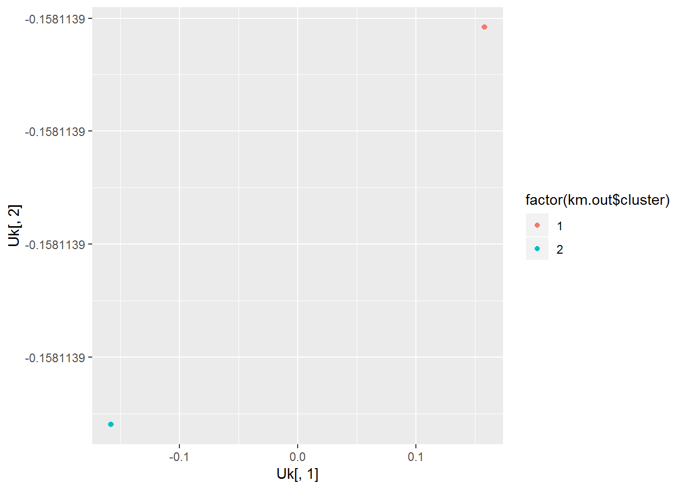
Result
Now we can look at the results in the original space. It got them perfectly as expected.
ggplot(data=x, mapping=aes(x=X1, y=X2, color=as.factor(km.out$cluster))) + geom_point()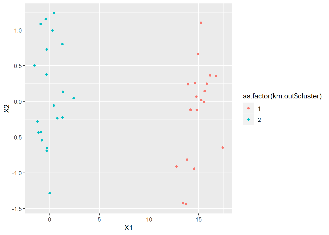
Making a function
Let’s put this all in a single function.
spec_cluster <- function(x, k, sig=.5) {
  N <- nrow(x)
  S <- outer(1:N, 1:N, Vectorize(function(i,j) {exp(-sum((x[i,1:2]-x[j,1:2])^2)/2/sig^2)}))
  W <- S
  D <- diag(rowSums(S))
  L <- D - W
  U <- eigen(L)$vec
  N <- nrow(x)
  Uk <- U[,(N-k+1):N]
  km.out <- kmeans(Uk, k)
  km.out$cluster
}
And another function that will just give us the plot instead of assignments when using 2D data.
plot_spec_cluster <- function(x, k, sig=.5) {
  assignments <- spec_cluster(x, k)
  sc.out <- spec_cluster(x,k)
  x <- data.frame(X1=x[,1], X2=x[,2], sig=sig)
  ggplot(data=x, mapping=aes(x=X1, y=X2, color=as.factor(sc.out))) + geom_point()
}
Try some examples
plot_spec_cluster(matrix(runif(100*2), ncol=2), 2)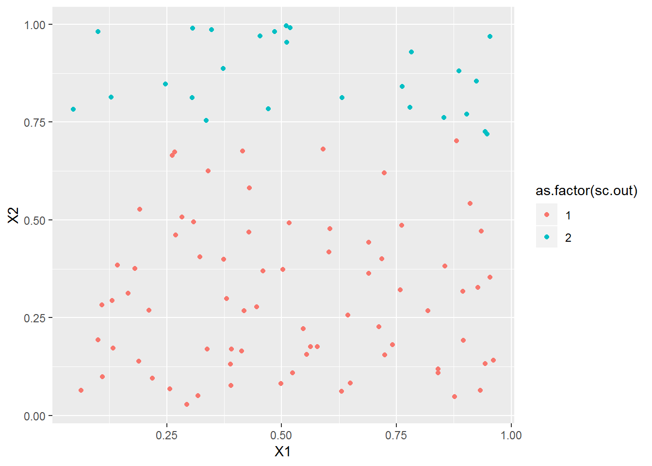
xl <- seq(0,1,l=51)
x2 <- cbind(xl, sin(2*pi*xl))
plot_spec_cluster(x2, 2)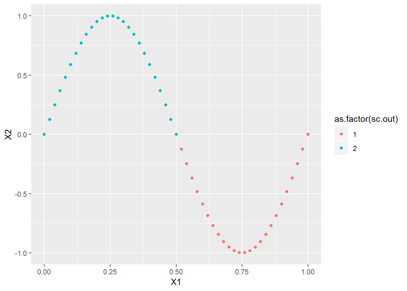
xl <- seq(0,1,l=51)
x2 <- cbind(xl, sin(2*pi*xl)) + rnorm(length(xl)*2, 0, .01)
plot_spec_cluster(x2, 2)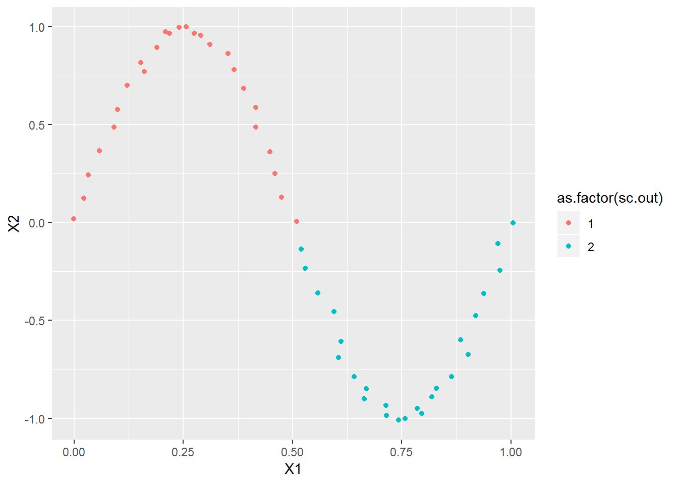
xl <- seq(0,1,l=251)
x2 <- cbind(xl, sin(2*pi*xl)*sample(c(-1,1),length(xl),T)) + rnorm(length(xl)*2, 0, .01)
plot_spec_cluster(x2, 2)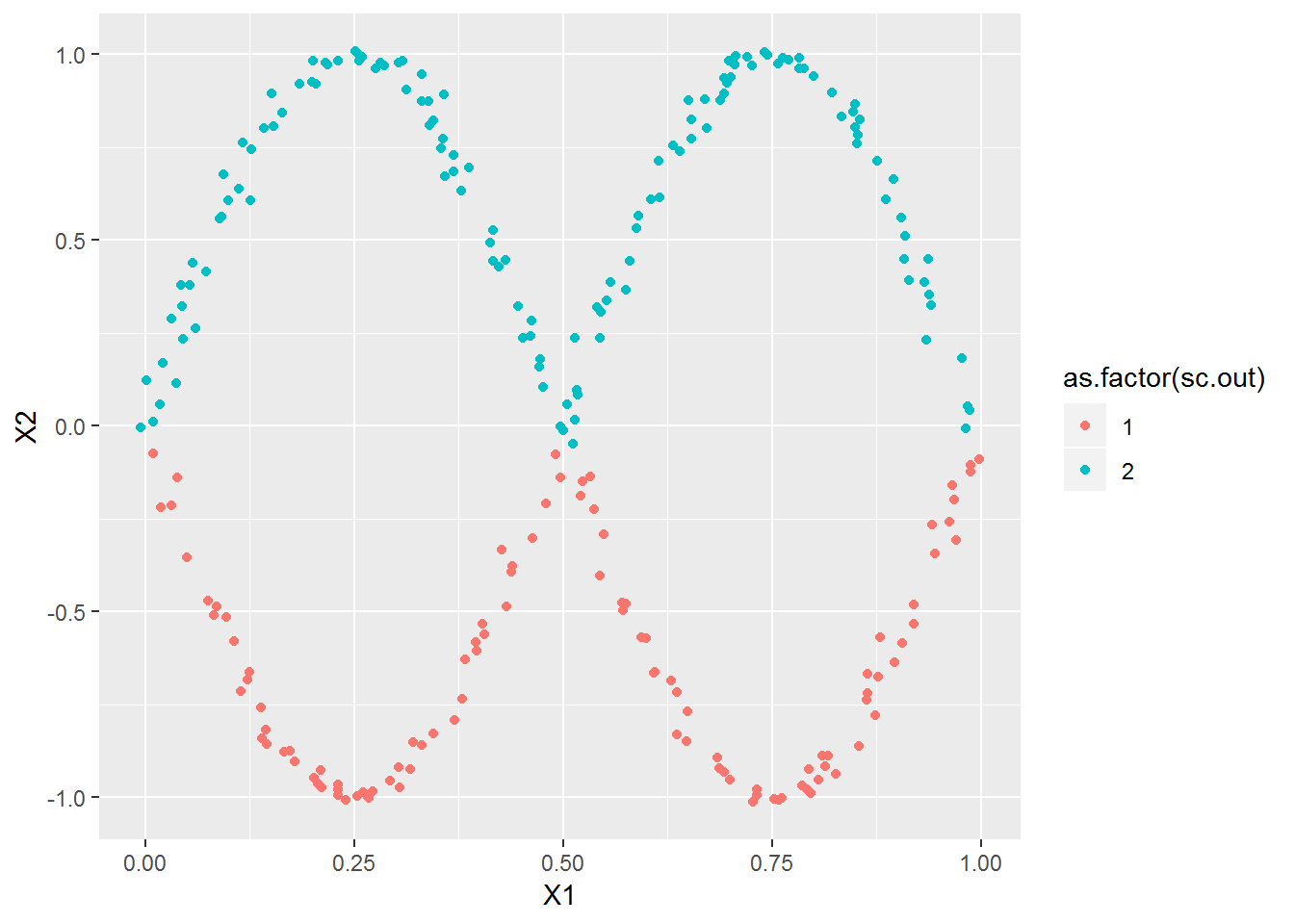
xl <- seq(0,1,l=251)
x2 <- cbind(xl, sin(2*pi*xl)) + rnorm(length(xl)*2, 0, .03)
x2[ceiling(length(xl)/2):length(xl),1] <- x2[ceiling(length(xl)/2):length(xl),1]-.25
plot_spec_cluster(x2, 2)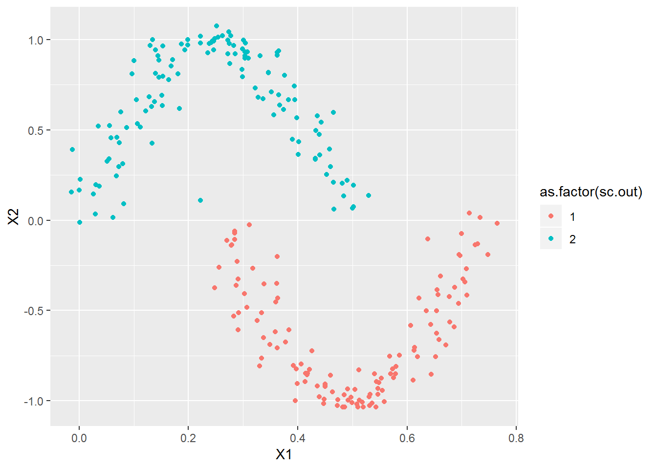
n1 <- 200
n2 <- 1000
xa <- cbind(rnorm(n1), rnorm(n1))
xb <- 3*cbind(rnorm(n2), rnorm(n2))
xb <- xb[rowSums(xb^2)>5^2,]
xb <- xb[rowSums(xb^2)<7^2,]
x2 <- rbind(xa,xb)
plot_spec_cluster(x2, 2, sig=2)
Summary
Spectral clustering appears to be one of the best clustering algorithm.
It works by finding the similarity between points and then using
eigenvectors to cluster these.
It can easily be implemented, the slowest part is finding eigenvectors.
This could be sped up from what I did before by using a function that only
finds the required eigenvectors, such as eigs in rARPACK.
There are many choices for the similarity function, and setting the parameters for these functions may cause issues. I had some trouble where a point would be put in a cluster with only itself because it was far from other points, even though it clearly belonged to one of the clusters. I think using a different similarity function, such as a nearest neighbor-based one, would do better and also avoid the issue of parameter tuning.