Once again I’m going to be trying something new, and mainly just using this blog post to track it for later reference. This time I am going to implement an autoencoder, and I’m going to use the R interface to TensorFlow to do it.
Data
I’m not going to use real data. I’m just going to creating a function that will give a sequence of numbers. These will be fed into the network, with the goal being to get the same thing out on the other side.
I’ll just use values from a sine function. Each training instance will have points generated from a different set of parameters. The parameters of a sine function are the phase, frequency, and amplitude.
Here’s what a single data instance will look like, I’ll evaluate the function at \(0, \ldots, 100\).
generate_instance <- function(x, phase, frequency, amplitude) {
  amplitude*sin(x*frequency-phase)
}
plot(generate_instance(0:100, 0, .1, 1.5))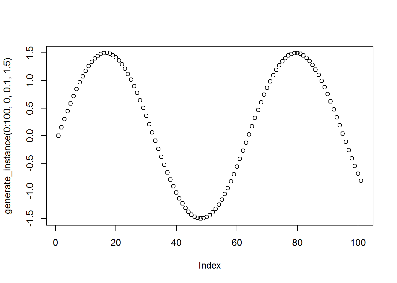
Here’s a function to get multiple instances, which will make it easy to generate a batch for training.
get_instances <- function(k) {
  sapply(1:k,
         function(xx) generate_instance(0:100, runif(1,0,100),runif(1, .03, .5),runif(1,.1,10))
         )
}
Here is a function that will make it easy to plot three input sets along with the model predictions.
plot_pairs <- function(x, y) {
  par(mfrow=c(1,3))
  for (i in 1:nrow(x)) {
    plot(x[i,], cex=1.4, ylab='')
    if (!missing(y)) points(y[i,], col=2, pch=4)
  }
}
Here are an example of what 3 randomly generated instances look like.
plot_pairs(t(get_instances(3)))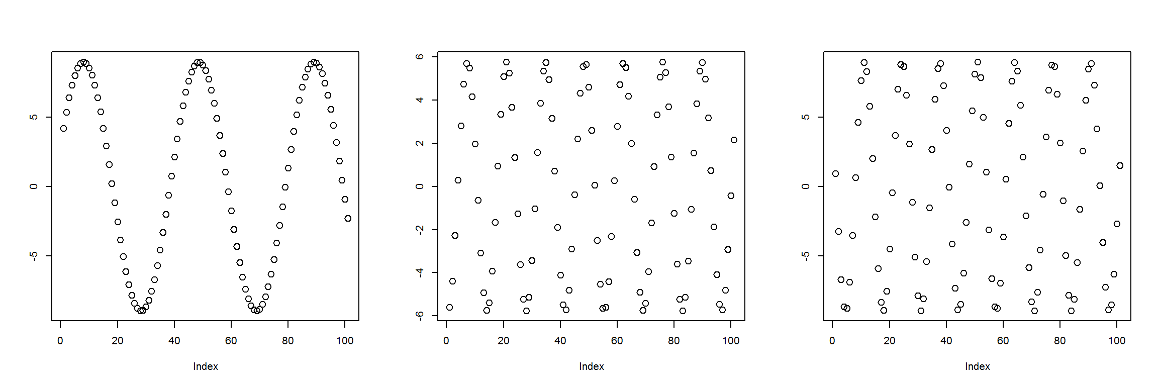
Autoencoder
The key idea of an autoencoder is that if we expect the output of a neural network to be equal to the input, and if there is a layer in the network with fewer nodes than the inputs, then the values at this layer represent a sort of data compression of the inputs.
So I’ll randomly generate function parameters (phase, frequency, and amplitude) to get a function, evaluate this function at a set of inputs, feed this into a neural network, and have the loss function be minimized when the outputs of the network are the same as the inputs.
Loss function
The loss function can just be the MSE (mean squared error). This will guide the neural network to make as close an approximation as possible over all the points.
TensorFlow code
I haven’t done much TensorFlow in R, I’ve done more in Python, so I’m just learning as I go along here. I’m going to look at some examples from here for guidance.
First I’ll do a trivial network, where the 101 inputs feed directly into the 101 outputs. It should learn to put 1 on the weights connecting straight across, and 0 everywhere else.
library(tensorflow)

X <- tf$placeholder(tf$float32, list(NULL, 101))
#dense1 <- tf$layers$dense(X, 101, activation = tf$sigmoid)
Out <- tf$layers$dense(X, 101) # Default activation is linear

mse <- tf$reduce_mean(tf$square(X - Out))
train_step <- tf$train$AdamOptimizer(1e-3)$minimize(mse)

sess <-  tf$Session()
sess$run(tf$global_variables_initializer())

N <- 2000
mses <- numeric(N)
for (i in 1:N) {
  batch <- t(get_instances(100))

  train_mse <- mse$eval(feed_dict = dict(
    X = batch), session = sess)
  mses[i] <- train_mse
  if (i %% 100 == 0) {
    cat(sprintf("step %d, training MSE %g\n", i, train_mse))
  }
  train_step$run(feed_dict = dict(X = batch), session = sess)
}
## step 100, training MSE 3.61996
## step 200, training MSE 0.754763
## step 300, training MSE 0.20967
## step 400, training MSE 0.0981752
## step 500, training MSE 0.0468911
## step 600, training MSE 0.0562941
## step 700, training MSE 0.0488362
## step 800, training MSE 0.0319513
## step 900, training MSE 0.023597
## step 1000, training MSE 0.0170169
## step 1100, training MSE 0.0153464
## step 1200, training MSE 0.0201433
## step 1300, training MSE 0.0114316
## step 1400, training MSE 0.0134869
## step 1500, training MSE 0.00827273
## step 1600, training MSE 0.00888674
## step 1700, training MSE 0.00854856
## step 1800, training MSE 0.00513882
## step 1900, training MSE 0.00623467
## step 2000, training MSE 0.00549583plot(mses, xlab="Batch number", ylab="MSE (log scale)", type='l', log='y')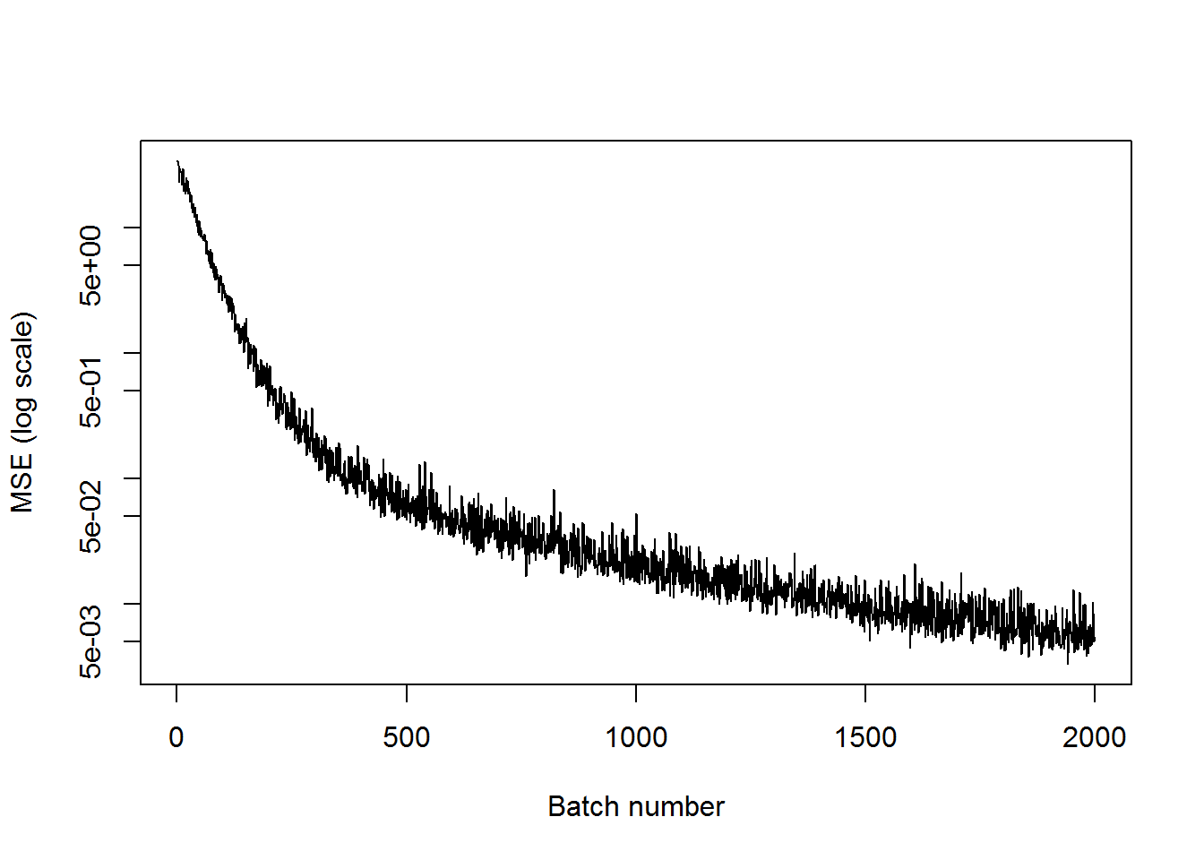
We can see that the training MSE has decreased significantly.
X1 <- t(get_instances(3))
preds <- sess$run(Out, feed_dict=dict(X=X1))
plot_pairs(X1, preds)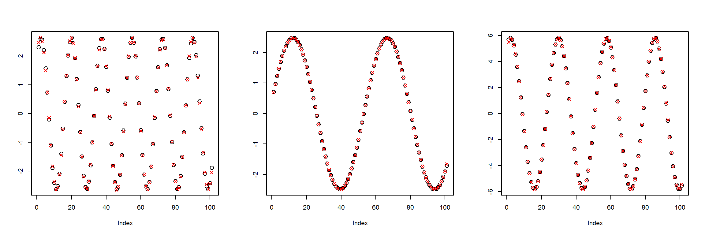
These sample plots show that the network gets the outputs almost exactly correct. Thus we have created a network that accomplishes the goal, but it can do this by simply passing the inputs straight to the outputs. What we want to do is add middle layers with fewer nodes so that the network has to perform a kind of data compression.
Adding another layer with 10 nodes in middle
Now I’ll try the same thing, except I’ll add a layer between the inputs and outputs with fewer nodes. Now the network will have to perform some sort of data compression to get the outputs to match the inputs. I’ll also let it run for more batches since it will be harder to learn the appropriate model weights.
The middle layer has 10 nodes and is densely connected between the inputs and outputs.
X <- tf$placeholder(tf$float32, list(NULL, 101))
dense1 <- tf$layers$dense(X, 10, activation = tf$sigmoid)
Out <- tf$layers$dense(dense1, 101) # Default activation is linear

mse <- tf$reduce_mean(tf$square(X - Out))
train_step <- tf$train$AdamOptimizer(1e-3)$minimize(mse)

sess <-  tf$Session()
sess$run(tf$global_variables_initializer())

N <- 10000
mses <- numeric(N)
for (i in 1:N) {
  batch <- t(get_instances(100))
  train_mse <- mse$eval(feed_dict = dict(
    X = batch), session = sess)
  mses[i] <- train_mse
  if (i %% 500 == 0) {
    cat(sprintf("step %d, training MSE %g\n", i, train_mse))
  }
  train_step$run(feed_dict = dict(X = batch), session = sess)
}
## step 500, training MSE 17.2054
## step 1000, training MSE 13.5368
## step 1500, training MSE 10.2691
## step 2000, training MSE 12.1905
## step 2500, training MSE 9.08547
## step 3000, training MSE 9.02409
## step 3500, training MSE 9.98993
## step 4000, training MSE 8.30779
## step 4500, training MSE 7.72379
## step 5000, training MSE 8.08216
## step 5500, training MSE 7.08383
## step 6000, training MSE 6.71515
## step 6500, training MSE 7.70897
## step 7000, training MSE 7.06879
## step 7500, training MSE 7.38318
## step 8000, training MSE 7.18005
## step 8500, training MSE 6.77941
## step 9000, training MSE 6.23073
## step 9500, training MSE 5.90885
## step 10000, training MSE 6.34011plot(mses, xlab="Batch number", ylab="MSE", type='l')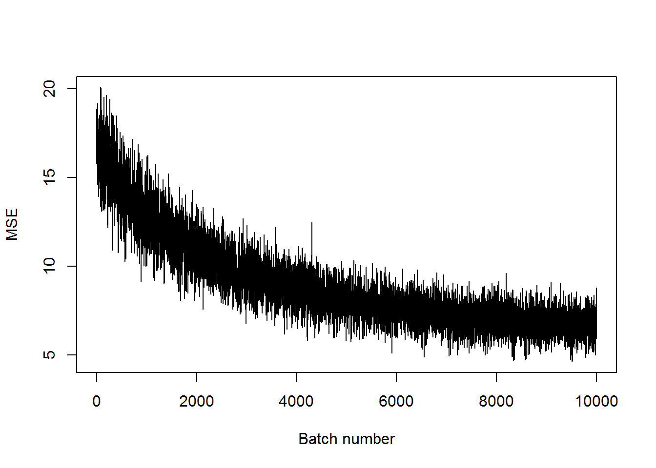
The MSE hasn’t gotten as small as before, but it has decreased a bit. It definitely will do better with more training. Let’s look at some of the examples to see what these look like with a fairly high MSE.
X1 <- t(get_instances(3))
preds <- sess$run(Out, feed_dict=dict(X=X1))
plot_pairs(X1, preds)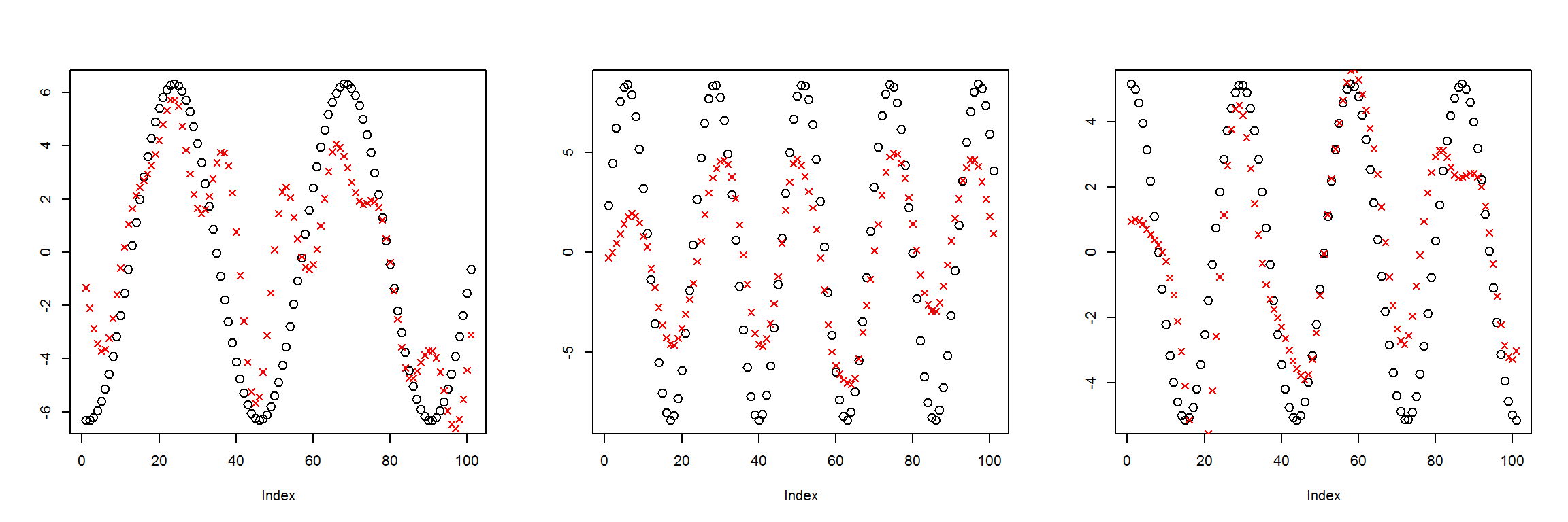
This model was clearly undertrained, I’ll try training it for longer.
X <- tf$placeholder(tf$float32, list(NULL, 101))
dense1 <- tf$layers$dense(X, 10, activation = tf$sigmoid)
Out <- tf$layers$dense(dense1, 101) # Default activation is linear

mse <- tf$reduce_mean(tf$square(X - Out))
train_step <- tf$train$AdamOptimizer(1e-3)$minimize(mse)

sess <-  tf$Session()
sess$run(tf$global_variables_initializer())

N <- 10000
mses <- numeric(N)
for (i in 1:N) {
  batch <- t(get_instances(100))
  train_mse <- mse$eval(feed_dict = dict(
    X = batch), session = sess)
  mses[i] <- train_mse
  if (i %% 5000 == 0) {
    cat(sprintf("step %d, training MSE %g\n", i, train_mse))
  }
  train_step$run(feed_dict = dict(X = batch), session = sess)
}
## step 5000, training MSE 8.82519
## step 10000, training MSE 6.6178plot(mses, xlab="Batch number", ylab="MSE", type='l')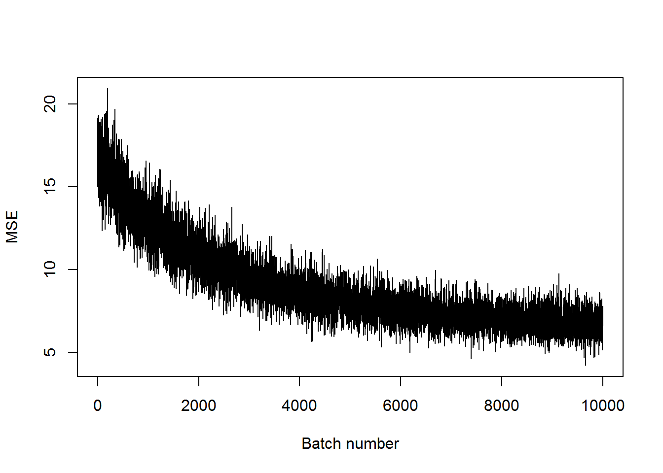
X1 <- t(get_instances(3))
preds <- sess$run(Out, feed_dict=dict(X=X1))
plot_pairs(X1, preds)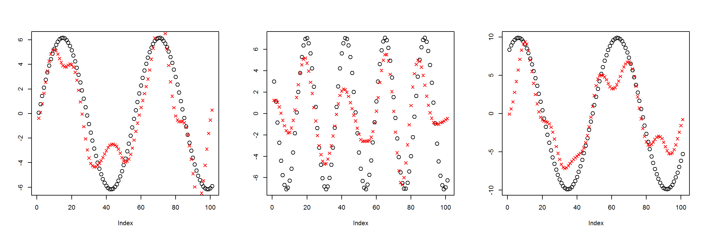
Add more layers again
X <- tf$placeholder(tf$float32, list(NULL, 101))
dense1 <- tf$layers$dense(X, 50, activation = tf$nn$selu)
dense2 <- tf$layers$dense(dense1, 10, activation = tf$nn$selu)
dense3 <- tf$layers$dense(dense2, 50, activation = tf$nn$selu)
Out <- tf$layers$dense(dense3, 101) # Default activation is linear

mse <- tf$reduce_mean(tf$square(X - Out))
train_step <- tf$train$AdamOptimizer(1e-3)$minimize(mse)

sess <-  tf$Session()
sess$run(tf$global_variables_initializer())

N <- 100000
mses <- numeric(N)
for (i in 1:N) {
  batch <- t(get_instances(100))
  train_mse <- mse$eval(feed_dict = dict(
    X = batch), session = sess)
  mses[i] <- train_mse
  if (i %% 5000 == 0) {
    cat(sprintf("step %d, training MSE %g\n", i, train_mse))
  }
  train_step$run(feed_dict = dict(X = batch), session = sess)
}
## step 5000, training MSE 0.342407
## step 10000, training MSE 0.149557
## step 15000, training MSE 0.113041
## step 20000, training MSE 0.139886
## step 25000, training MSE 0.104381
## step 30000, training MSE 0.0879787
## step 35000, training MSE 0.074021
## step 40000, training MSE 0.0724682
## step 45000, training MSE 0.0875358
## step 50000, training MSE 0.0627108
## step 55000, training MSE 0.0768229
## step 60000, training MSE 0.0798857
## step 65000, training MSE 0.0624588
## step 70000, training MSE 0.0651367
## step 75000, training MSE 0.0614307
## step 80000, training MSE 0.0554227
## step 85000, training MSE 0.0792781
## step 90000, training MSE 0.0499048
## step 95000, training MSE 0.0587971
## step 100000, training MSE 0.0429378plot(mses, xlab="Batch number", ylab="MSE (log scale)", type='l', log='y')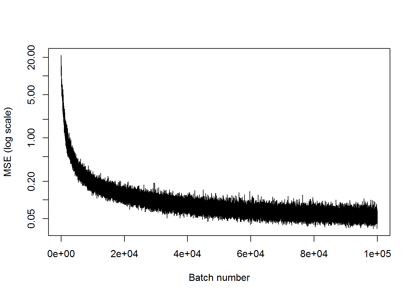
X1 <- t(get_instances(3))
preds <- sess$run(Out, feed_dict=dict(X=X1))
plot_pairs(X1, preds)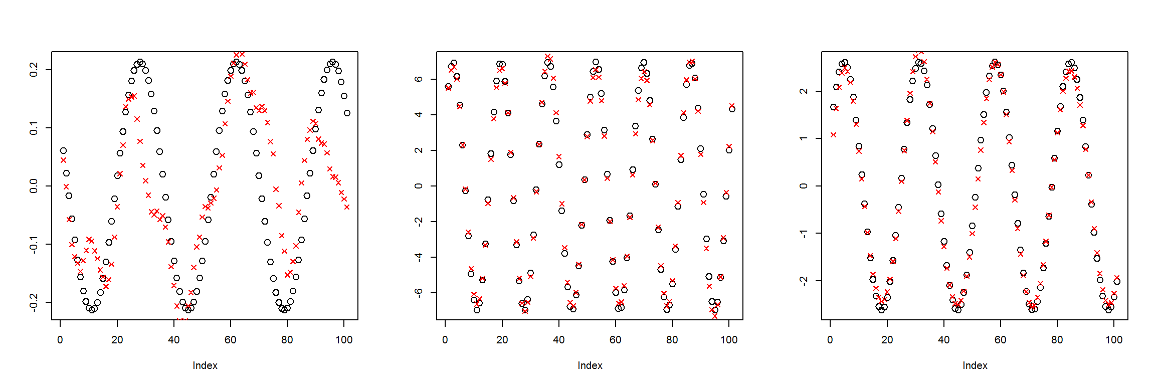
We can see this network has learned to recreate the 101 inputs with only 10 nodes in the middle layer decently well. This means that the information was compressed to be 1/10 of its original size. There is a bit of a difference in the first example, but the latter two look much better.
A middle layer with only 3 nodes
Since the data is created using three parameters (frequency, amplitude, and phase), we should be able to recreated the inputs even if there is a middle layer with as few as 3 nodes.
This will likely take longer to train, and maybe need more intermediate layers to calculate the required information. First I’ll just run it with the same 101-50-3-50-101 structure to see how it does.
X <- tf$placeholder(tf$float32, list(NULL, 101))
dense1 <- tf$layers$dense(X, 50, activation = tf$nn$selu)
dense2 <- tf$layers$dense(dense1, 3, activation = tf$nn$selu)
dense3 <- tf$layers$dense(dense2, 50, activation = tf$nn$selu)
Out <- tf$layers$dense(dense3, 101) # Default activation is linear

mse <- tf$reduce_mean(tf$square(X - Out))
train_step <- tf$train$AdamOptimizer(1e-3)$minimize(mse)

sess <-  tf$Session()
sess$run(tf$global_variables_initializer())

N <- 100000
mses <- numeric(N)
for (i in 1:N) {
  batch <- t(get_instances(100))
  train_mse <- mse$eval(feed_dict = dict(
    X = batch), session = sess)
  mses[i] <- train_mse
  if (i %% 5000 == 0) {
    cat(sprintf("step %d, training MSE %g\n", i, train_mse))
  }
  train_step$run(feed_dict = dict(X = batch), session = sess)
}
## step 5000, training MSE 8.47767
## step 10000, training MSE 5.27897
## step 15000, training MSE 4.4829
## step 20000, training MSE 3.9965
## step 25000, training MSE 4.13361
## step 30000, training MSE 3.34761
## step 35000, training MSE 2.73894
## step 40000, training MSE 3.01699
## step 45000, training MSE 4.4124
## step 50000, training MSE 2.62927
## step 55000, training MSE 2.15425
## step 60000, training MSE 3.19839
## step 65000, training MSE 3.18557
## step 70000, training MSE 3.16618
## step 75000, training MSE 2.22587
## step 80000, training MSE 2.92989
## step 85000, training MSE 2.33331
## step 90000, training MSE 3.31358
## step 95000, training MSE 3.08208
## step 100000, training MSE 2.4895plot(mses, xlab="Batch number", ylab="MSE (log scale)", type='l', log='y')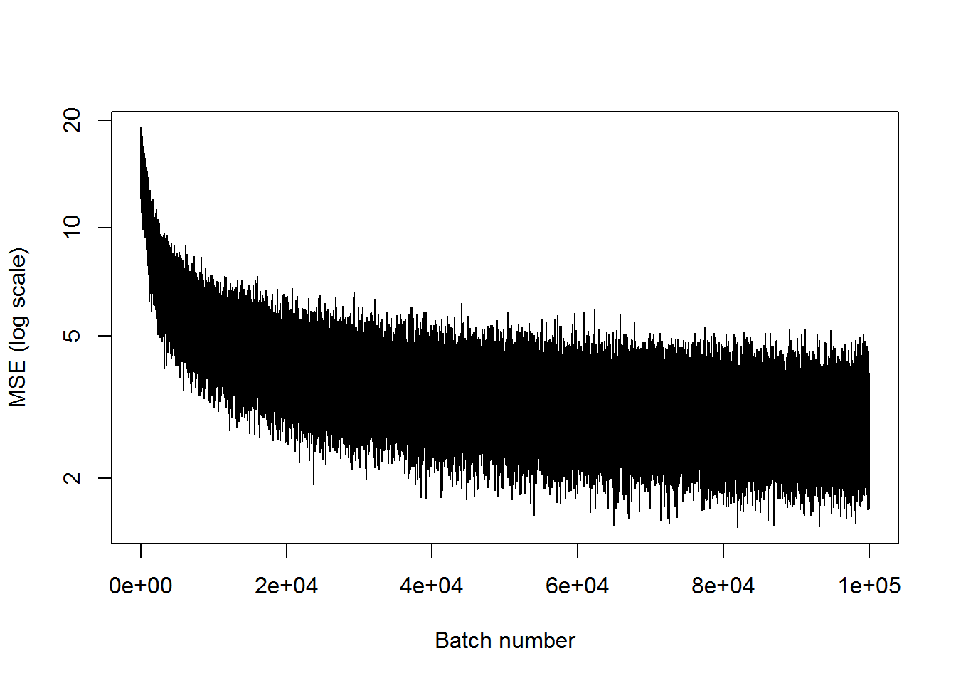
X1 <- t(get_instances(6))
preds <- sess$run(Out, feed_dict=dict(X=X1))
plot_pairs(X1, preds)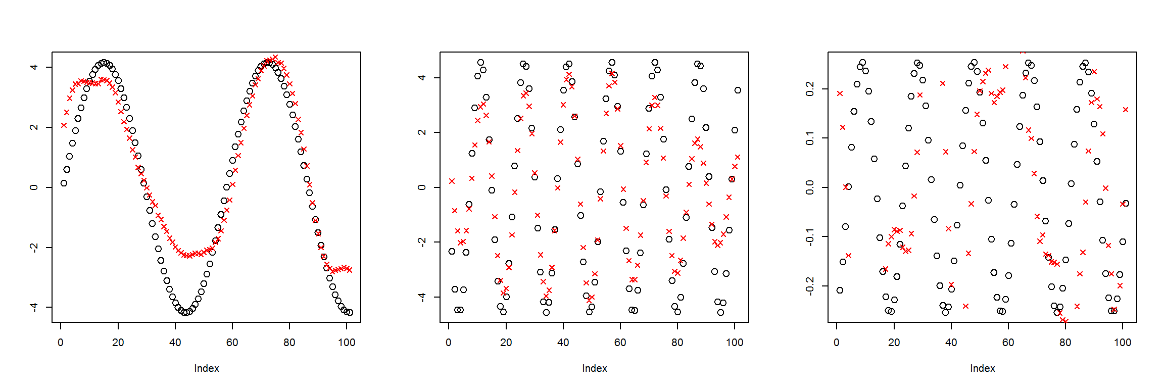
This is not that good. The network probably needs more layers in order to calculate the useful parameters in the middle layer that can be used to recreate the inputs.
Adding more layers, still 3 nodes in middle
The MSE had leveled out but the accuracies weren’t that great in the last example. It may be that it needs more layers in order to compress the function parameters into the three nodes of the middle layer.
X <- tf$placeholder(tf$float32, list(NULL, 101))
dense1 <- tf$layers$dense(X, 50, activation = tf$nn$selu)
dense1b <- tf$layers$dense(dense1, 20, activation = tf$nn$selu)
dense2 <- tf$layers$dense(dense1b, 3, activation = tf$nn$selu)
dense2b <- tf$layers$dense(dense2, 20, activation = tf$nn$selu)
dense3 <- tf$layers$dense(dense2b, 50, activation = tf$nn$selu)
Out <- tf$layers$dense(dense3, 101) # Default activation is linear

mse <- tf$reduce_mean(tf$square(X - Out))
train_step <- tf$train$AdamOptimizer(1e-3)$minimize(mse)

sess <-  tf$Session()
sess$run(tf$global_variables_initializer())

N <- 100000
mses <- numeric(N)
for (i in 1:N) {
  batch <- t(get_instances(100))
  train_mse <- mse$eval(feed_dict = dict(
    X = batch), session = sess)
  mses[i] <- train_mse
  if (i %% 5000 == 0) {
    cat(sprintf("step %d, training MSE %g\n", i, train_mse))
  }
  train_step$run(feed_dict = dict(X = batch), session = sess)
}
## step 5000, training MSE 2.83734
## step 10000, training MSE 1.582
## step 15000, training MSE 1.31236
## step 20000, training MSE 1.14391
## step 25000, training MSE 0.911683
## step 30000, training MSE 0.654616
## step 35000, training MSE 1.18588
## step 40000, training MSE 0.931521
## step 45000, training MSE 0.765716
## step 50000, training MSE 0.81019
## step 55000, training MSE 0.912352
## step 60000, training MSE 1.28228
## step 65000, training MSE 0.923536
## step 70000, training MSE 0.790987
## step 75000, training MSE 0.665161
## step 80000, training MSE 0.784157
## step 85000, training MSE 0.849936
## step 90000, training MSE 0.410614
## step 95000, training MSE 0.59526
## step 100000, training MSE 0.756836plot(mses, xlab="Batch number", ylab="MSE (log scale)", type='l', log='y')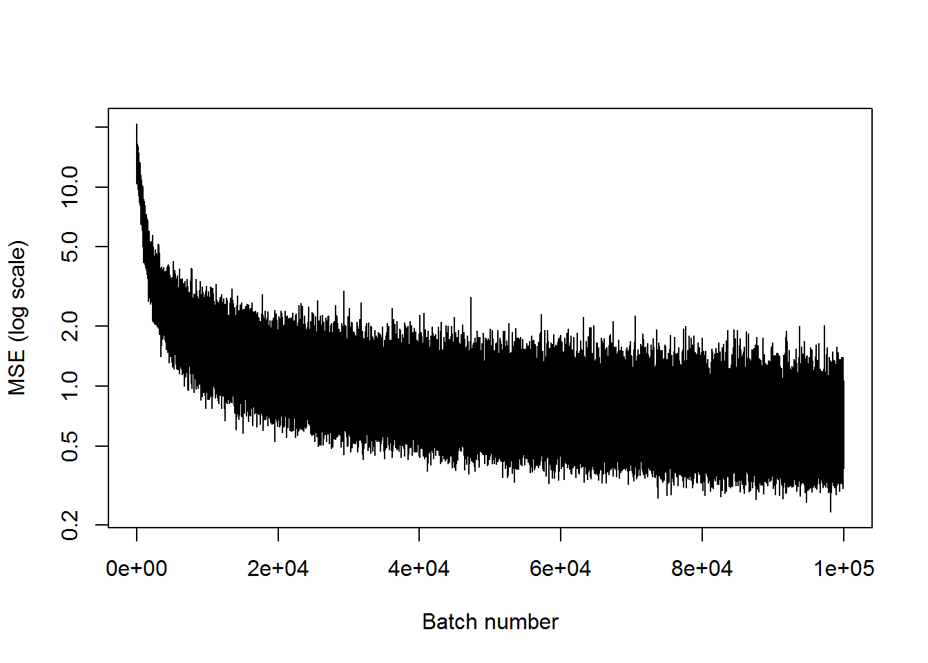
X1 <- t(get_instances(6))
preds <- sess$run(Out, feed_dict=dict(X=X1))
plot_pairs(X1, preds)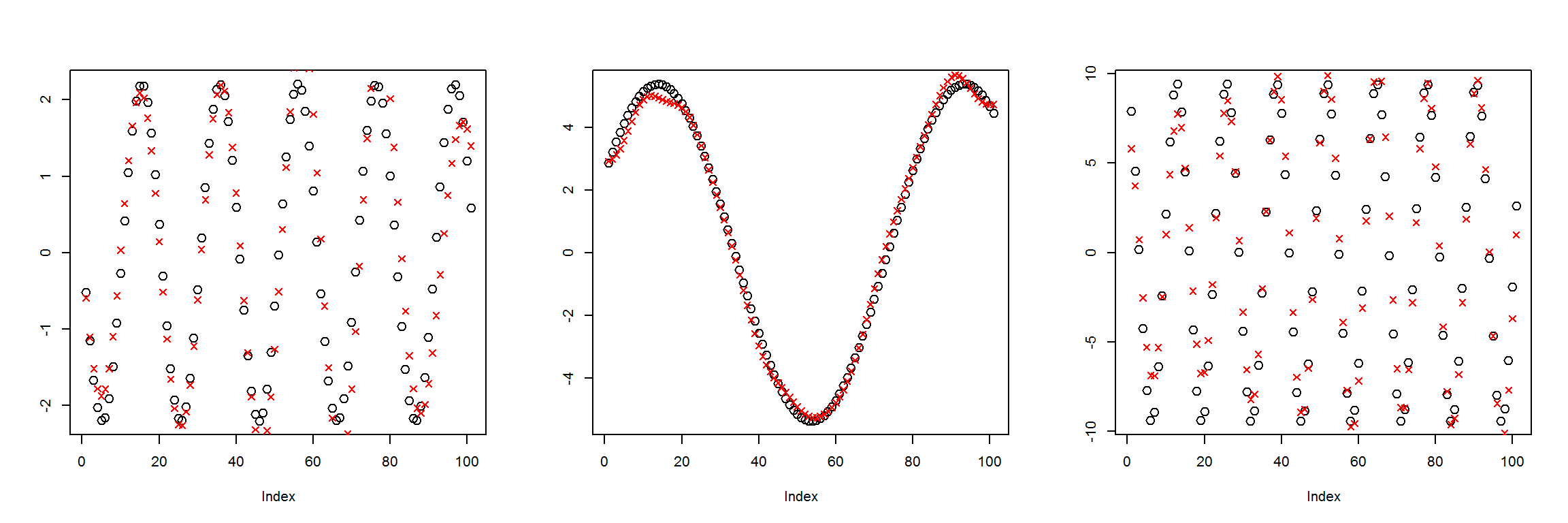
This has an MSE of about 1, compared to 3 for the last case. So it’s getting better, but still not great. I’m going to try to add another pair of inner layers, and see if that does the trick.
More layers with 3 nodes in the middle
X <- tf$placeholder(tf$float32, list(NULL, 101))
dense1 <- tf$layers$dense(X, 50, activation = tf$nn$selu)
dense1b <- tf$layers$dense(dense1, 20, activation = tf$nn$selu)
dense1c <- tf$layers$dense(dense1b, 10, activation = tf$nn$selu)
dense2 <- tf$layers$dense(dense1c, 3, activation = tf$nn$selu)
dense2b <- tf$layers$dense(dense2, 10, activation = tf$nn$selu)
dense2c <- tf$layers$dense(dense2b, 20, activation = tf$nn$selu)
dense3 <- tf$layers$dense(dense2c, 50, activation = tf$nn$selu)
Out <- tf$layers$dense(dense3, 101) # Default activation is linear

mse <- tf$reduce_mean(tf$square(X - Out))
train_step <- tf$train$AdamOptimizer(1e-3)$minimize(mse)

sess <-  tf$Session()
sess$run(tf$global_variables_initializer())

N <- 100000
mses <- numeric(N)
for (i in 1:N) {
  batch <- t(get_instances(100))
  train_mse <- mse$eval(feed_dict = dict(
    X = batch), session = sess)
  mses[i] <- train_mse
  if (i %% 5000 == 0) {
    cat(sprintf("step %d, training MSE %g\n", i, train_mse))
  }
  train_step$run(feed_dict = dict(X = batch), session = sess)
}
## step 5000, training MSE 2.3947
## step 10000, training MSE 2.22703
## step 15000, training MSE 1.45675
## step 20000, training MSE 1.36512
## step 25000, training MSE 1.45944
## step 30000, training MSE 1.36662
## step 35000, training MSE 1.59973
## step 40000, training MSE 1.12988
## step 45000, training MSE 1.25019
## step 50000, training MSE 0.83034
## step 55000, training MSE 1.34451
## step 60000, training MSE 0.736481
## step 65000, training MSE 1.75069
## step 70000, training MSE 1.02848
## step 75000, training MSE 0.921248
## step 80000, training MSE 0.680152
## step 85000, training MSE 0.754047
## step 90000, training MSE 1.37079
## step 95000, training MSE 0.871477
## step 100000, training MSE 0.439818plot(mses, xlab="Batch number", ylab="MSE (log scale)", type='l', log='y')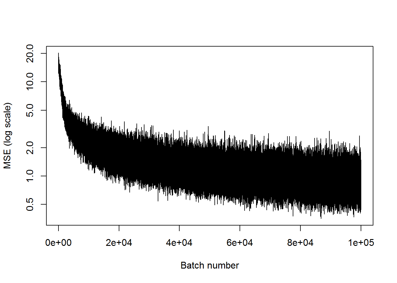
X1 <- t(get_instances(6))
preds <- sess$run(Out, feed_dict=dict(X=X1))
plot_pairs(X1, preds)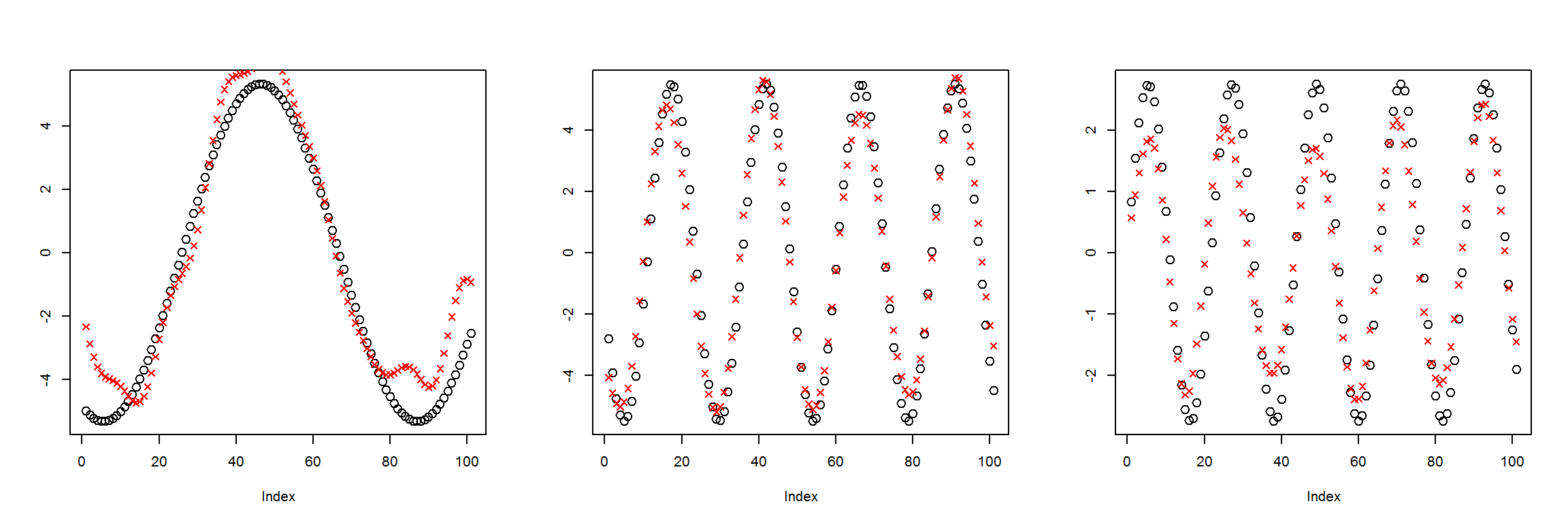
This is about as good as the last one. The MSE leveled out around 1, and there are clear deviations between the inputs and the outputs.
Two nodes in the middle layer
My hypothesis was that the outputs could recreate the inputs with as few as three nodes in the middle layer. I showed that with 3 nodes in the middle layer, it does a pretty good job. Now I want to see what will happen with only two nodes in the middle layer.
With only two nodes in the middle layer, the network won’t be able to keep information for three independent parameters. Let’s see how it does with the same network, with the only difference being reducing the middle layer nodes from three to two.
X <- tf$placeholder(tf$float32, list(NULL, 101))
dense1 <- tf$layers$dense(X, 50, activation = tf$nn$selu)
dense1b <- tf$layers$dense(dense1, 20, activation = tf$nn$selu)
dense1c <- tf$layers$dense(dense1b, 10, activation = tf$nn$selu)
dense2 <- tf$layers$dense(dense1c, 2, activation = tf$nn$selu)
dense2b <- tf$layers$dense(dense2, 10, activation = tf$nn$selu)
dense2c <- tf$layers$dense(dense2b, 20, activation = tf$nn$selu)
dense3 <- tf$layers$dense(dense2c, 50, activation = tf$nn$selu)
Out <- tf$layers$dense(dense3, 101) # Default activation is linear

mse <- tf$reduce_mean(tf$square(X - Out))
train_step <- tf$train$AdamOptimizer(1e-3)$minimize(mse)

sess <-  tf$Session()
sess$run(tf$global_variables_initializer())

N <- 100000
mses <- numeric(N)
for (i in 1:N) {
  batch <- t(get_instances(100))
  train_mse <- mse$eval(feed_dict = dict(
    X = batch), session = sess)
  mses[i] <- train_mse
  if (i %% 5000 == 0) {
    cat(sprintf("step %d, training MSE %g\n", i, train_mse))
  }
  train_step$run(feed_dict = dict(X = batch), session = sess)
}
## step 5000, training MSE 7.0935
## step 10000, training MSE 5.73481
## step 15000, training MSE 5.4371
## step 20000, training MSE 4.55731
## step 25000, training MSE 4.96801
## step 30000, training MSE 5.46502
## step 35000, training MSE 3.48382
## step 40000, training MSE 4.26079
## step 45000, training MSE 4.00776
## step 50000, training MSE 4.65524
## step 55000, training MSE 3.38982
## step 60000, training MSE 4.40078
## step 65000, training MSE 5.05162
## step 70000, training MSE 4.60735
## step 75000, training MSE 3.81621
## step 80000, training MSE 4.04185
## step 85000, training MSE 3.26245
## step 90000, training MSE 3.43061
## step 95000, training MSE 3.15188
## step 100000, training MSE 3.82056plot(mses, xlab="Batch number", ylab="MSE (log scale)", type='l', log='y')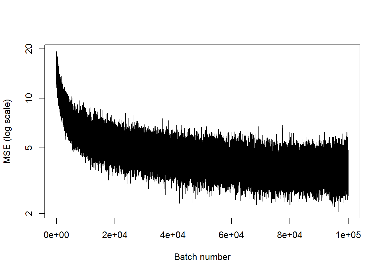
X1 <- t(get_instances(6))
preds <- sess$run(Out, feed_dict=dict(X=X1))
plot_pairs(X1, preds)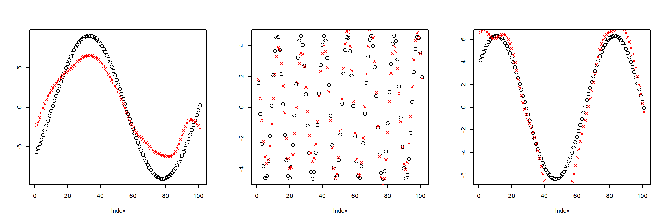
It’s definitely worse than when there were three nodes in the middle layer, but it’s not nearly as bad as expected.
Conclusion
In this post I have tried to create an autoencoder for sequences of sinusoidal data using TensorFlow in R. Autoencoders essentially work as a data compression algorithm. By forcing the data through a neural network that is skinny in the middle, the nodes in the skinniest layer must attempt to carry as much information as possible in order to recreate the inputs.
I only tried to do a very basic version. For future tests I’d like to try to implement an autoencoder on a more useful data set. I should also look into what tools TensorFlow may provide for creating autoencoders, or check out other blog posts from other people. I did all this with only a very basic idea of what autoencoders do, so I’m sure I’m missing a lot of details.