There’s a somewhat famous blog post titled Don’t Invert That Matrix. This topic has also been discussed using R on this blog post. You should read those instead of this. I’m just experimenting to see how important this concept is in R, especially in the cases I use often.
The main idea
Often finding the inverse of a matrix is not the endgoal. If it is, then you have do invert it. Otherwise you are usually trying to solve a system of equations, \(Ax=b\), for the vector \(x\), where \(A\) is a matrix and \(b\) is a given vector. You may need to solve this for many different \(b\) or for a single one. If you only need to solve it for a single \(b\), you can simply run solve(A, b) and you are done.
It becomes more of an issue when you need to solve the equation for many different \(b\). Using solve is an \(O(n^3)\) operation, where \(n\) is the number of rows of \(A\), meaning it is slow. In small dimensions, you can just invert \(A\) by storing the result of solve(A), and multiplying this by each \(b\). If you have all your \(b\)’s at once, say in matrix \(B\), you can use solve(A, B) and you are done. So now the problem is really that you need to solve the equation for many different \(b\), and you don’t have all the \(b\)’s in the beginning, and that \(A\) is big. Think of having to solve an iterative equation.
Having to do an \(O(n^3)\) operation repeatedly is slow and a waste of resources. You could invert \(A\) once, then multiply that inverse times each \(b\) when needed. The problem with this is that calculating the inverse is not as numerically stable as factorizing the matrix.
Factoring a matrix
Factoring a matrix means you find matrices whose product is equal to \(A\). An LU-decomposition (Matrix::lu) finds a lower triangular matrix \(L\) and an upper triangular matrix \(U\) such that \(LU=A\). If \(A\) is not square, then it can be factored as \(A=PLU\). If \(A\) as symmetric and positive definite, then the Cholesky factorization (chol) gives an upper triangular matrix \(R\) such that \(R^T R = A\). Other matrix decompositions include QR factorization and SVD.
Once you have a factorization of \(A\), you can use the factors for each \(b\) to solve the system. Usually the factors are triangular or diagonal. The benefit of doing this is that it is much more numerically stable to solve using the factors then with the full inverse of \(A\).
Testing with correlation matrices
I’m going to use correlation matrices to test this, since that is what I use for Gaussian process models. These matrices are positive definite, so I can use the Cholesky decomposition. Below I create a 100x100 correlation matrix and plot it.
set.seed(0)
d <- 4
n <- 100
theta <- 2 #c(.05,.1,.05,1)
X <- matrix(runif(d*n), ncol=d)
A <- outer(1:n, 1:n,
           Vectorize(
             function(i,j) {
               exp(-sum(theta*(X[i,]-X[j,])^2))
             }
           ))
image(A)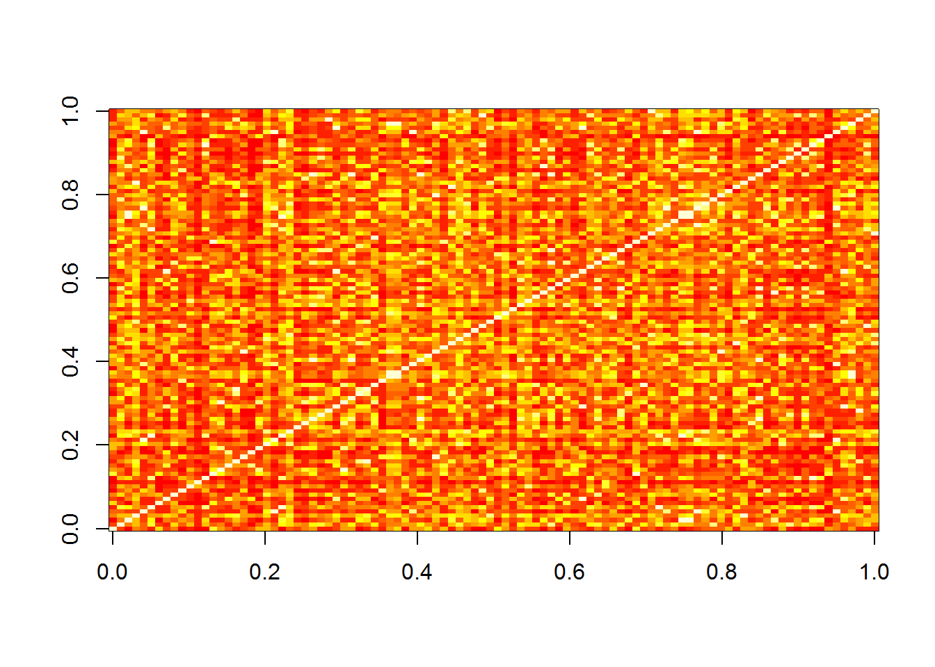
To see how poorly conditioned it is, we can check the eigenvalues.
summary(eigen(A, only.values = T)$values)## Min. 1st Qu. Median Mean 3rd Qu. Max.
## 0.00003 0.00169 0.01744 1.00000 0.23363 38.44173The smallest eigenvalue is about 0.00003, which is not great. The determinant of the \(A\) is 2.07338210^{-170}, which makes me think it is poorly conditioned.
To see how the accuracy of the solve is, I’ll create a random vector \(x\) and calculate \(b\).
set.seed(1)
x <- rnorm(100)
b <- A %*% x
First we’ll check the difference between x and using solve.
summary(solve(A, b) - x)## V1
## Min. :-3.262e-11
## 1st Qu.:-1.552e-12
## Median :-8.965e-14
## Mean :-4.600e-16
## 3rd Qu.: 1.378e-12
## Max. : 2.962e-11Largest difference is about 3e-11.
Now we can see how far off the solution is when using the inverse compared to the correct answer.
A_inv <- solve(A)
summary(A_inv %*% b - x)
## V1
## Min. :-1.048e-10
## 1st Qu.:-6.826e-12
## Median :-7.054e-13
## Mean :-1.248e-13
## 3rd Qu.: 8.203e-12
## Max. : 1.142e-10The largest error is about 1.1e-10, which is 3x larger than when using solve.
Now using backsolve twice with the Cholesky factorization:
A_chol <- chol(A)
summary(backsolve(A_chol, backsolve(A_chol, b, transpose = T)) - x)
## V1
## Min. :-2.092e-11
## 1st Qu.:-1.043e-12
## Median : 5.845e-14
## Mean :-2.980e-16
## 3rd Qu.: 1.452e-12
## Max. : 1.790e-11Differences are as large as 2e-11, which is even smaller than when using solve.
How about LU decomposition? I tried first using Matrix::lu, but had issues. Instead I used matrixcalc::lu.decomposition.
library(matrixcalc)
A_lu <- lu.decomposition(A)
summary(c(A_lu$L %*% A_lu$U - A))
## Min. 1st Qu. Median Mean 3rd Qu. Max.
## -7.772e-16 -5.551e-17 0.000e+00 3.841e-19 5.551e-17 7.772e-16# Check that decomposition is correct, all < 1e-15
summary(backsolve(A_lu$U, backsolve(A_lu$L, b, upper.tri=F)) - x)## V1
## Min. :-3.248e-11
## 1st Qu.:-1.627e-12
## Median : 2.096e-14
## Mean :-3.500e-16
## 3rd Qu.: 1.319e-12
## Max. : 2.727e-11The biggest errors are about 3e-11, which is about the same as using solve, better than using the inverse, and worse than using Cholesky.
So far it seems that doing the full inverse is the least accurate, while the decompositions are about as accurate as using solve.
Using Hilbert matrices
The symmetric Hilbert matrices are known for being numerically unstable. I tried to invert the 20x20 Hilbert matrix, but R gave an error. The largest that is invertible is the 11x11.
set.seed(2)
n <- 11
A <- matrix(Matrix::Hilbert(n), n, n)
x <- rnorm(n)
b <- A %*% x
Using solve, the max error is about 6e-3.
summary(solve(A, b) - x)## V1
## Min. :-4.988e-03
## 1st Qu.:-5.101e-04
## Median :-3.000e-09
## Mean : 0.000e+00
## 3rd Qu.: 1.040e-03
## Max. : 5.973e-03Finding the inverse, the max error is about 2e-2, so about three times larger.
A_inv <- solve(A)
summary(A_inv %*% b - x)
## V1
## Min. :-0.0210056
## 1st Qu.:-0.0058718
## Median :-0.0004449
## Mean :-0.0004714
## 3rd Qu.: 0.0035936
## Max. : 0.0171158Using Cholesky, it is half as much as solve, 1e-2.
A_chol <- chol(A)
summary(backsolve(A_chol, backsolve(A_chol, b, transpose = T)) - x)
## V1
## Min. :-8.487e-03
## 1st Qu.:-8.691e-04
## Median :-5.000e-09
## Mean : 0.000e+00
## 3rd Qu.: 1.773e-03
## Max. : 1.017e-02And with LU decomposition the max error is half as large as that, 4e-3, or a little better than solve.
A_lu <- lu.decomposition(A)
summary(c(A_lu$L %*% A_lu$U - A))
## Min. 1st Qu. Median Mean 3rd Qu. Max.
## -2.776e-17 0.000e+00 0.000e+00 1.147e-19 0.000e+00 2.776e-17# Check that decomposition is correct, all < 1e-16
summary(backsolve(A_lu$U, backsolve(A_lu$L, b, upper.tri=F)) - x)## V1
## Min. :-3.328e-03
## 1st Qu.:-3.426e-04
## Median :-2.000e-09
## Mean : 0.000e+00
## 3rd Qu.: 7.016e-04
## Max. : 3.998e-03We are getting much larger errors than with the correlation matrix, up to about 1e-2 instead of 1e-11. This means that the conditioning of the matrix has a large effect on how accurate these solves are.
Again we see that finding the inverse is the least stable calculation, but not by a huge margin.
Downside of using decomposition
One downside of using the decomposition instead of the inverse is that it is a bit harder to use in calculations. Instead of A_inv %*% b, you have to do backsolve(A_chol, backsolve(A_chol, b, transpose = T)). You would probably want to write a function for it, or just create a new class.
A second downside is that it is slower. So if you only have to factor a matrix once, but solve the system of equations for hundreds of b’s, it may take way longer. Below is a benchmark comparing the times of using the inverse vs the Cholesky factorization vs the LU factorization.
microbenchmark::microbenchmark(
  A_inv %*% b,
  backsolve(A_chol, backsolve(A_chol, b, transpose = T)),
  backsolve(A_lu$U, backsolve(A_lu$L, b, upper.tri=F))
)
## Unit: nanoseconds
## expr min lq
## A_inv %*% b 380 380
## backsolve(A_chol, backsolve(A_chol, b, transpose = T)) 9123 9883
## backsolve(A_lu$U, backsolve(A_lu$L, b, upper.tri = F)) 9883 10263
## mean median uq max neval cld
## 661.49 760 760.5 3421 100 a
## 10711.72 10263 10643.0 23947 100 b
## 12467.75 11023 11404.0 61578 100 cUsing the inverse once you have it is over 10 times faster, a significant speedup. I thought in the past this was more like 2, it probably depends on the size of the matrix.
Summary
In summary, you should never invert a matrix. You either use solve to solve a single set of equations, or use a matrix decomposition for stability. However, it doesn’t seem like a huge difference numerically, and it can be a lot slower, so there are cases where you may just want to get the full inverse.