Generally neural networks act as black boxes. The input goes in, you get output, and there is interpretation of the data that helps you understand the model.
A gray box means that we impose structure on the internal structure of the neural network, so that after the model is fit we can look at the estimated parameters and they will tell us something useful.
One way we can do this is to encode an equation that we want to use near the end of the neural network.
For example, if I know that \(y=a e^{cx} + b\), I can have \(c\) be a variable, multiply \(x\) by it, use the exponential as the activation function, then do a linear layer to the output.
I will try to implement this example by adapting the linear regression model found here. The only changes I make are to add a third variable and change the equation for linear_model, now called exp_model. I also made minor changes such as changing the loss from sum to mean, and the print out.
I am using Python for this instead of R to make that I have all of the functionality. I’m writing this in RStudio as a Rmarkdown notebook, which conveniently lets you run Python code.
First model
The first two lines of code are just to hide the warnings from TF which get annoying quickly as recommended here. Notice that I have to have this, as well as the loading code such as import tensorflow as tf in every chunk. I guess Python chunks are all run separately.
import os
os.environ['TF_CPP_MIN_LOG_LEVEL']='2'
import numpy as np
import tensorflow as tf

# Model parameters
a = tf.Variable([.3], dtype=tf.float32)
b = tf.Variable([-.3], dtype=tf.float32)
c = tf.Variable([-.3], dtype=tf.float32)
# Model input and output
x = tf.placeholder(tf.float32)
exp_model = a * tf.exp(c * x) + b
y = tf.placeholder(tf.float32)
# loss
loss = tf.reduce_mean(tf.square(exp_model - y)) # sum of the squares
# optimizer
optimizer = tf.train.GradientDescentOptimizer(0.01)
train = optimizer.minimize(loss)
# training data
x_train = [1,2,3,4]
y_train = [0,-1,-2,-3]
# training loop
init = tf.global_variables_initializer()
sess = tf.Session()
sess.run(init) # reset values to wrong
for i in range(1000):
  sess.run(train, {x:x_train, y:y_train})

# evaluate training accuracy
#curr_W, curr_b, curr_loss = sess.run([W, b, loss], {x:x_train, y:y_train})
#print("W: %s b: %s loss: %s"%(curr_W, curr_b, curr_loss))
curr_a, curr_b, curr_c, curr_loss = sess.run([a, b, c, loss], {x:x_train, y:y_train})
sess.close()
print("a: %s \nb: %s \nc: %s \nloss: %s"%(curr_a, curr_b, curr_c, curr_loss))
## a: [ 2.57894111]
## b: [-2.33267903]
## c: [-0.494257]
## loss: 0.457323Let me check these values to see how well it matches the data.
x <- c(1, 2, 3, 4)
y <- c(0, -1, -2, -3)
plot(x, y)

a <- 5.4532733
b <- -3.58833456
c <- -.42571044
curve(a*exp(c*x) + b, add=T, col=2)
This actually looks pretty good considering that we forced the model to be nonlinear for data that is exactly linear.
Using data from an exponential function.
I’ll try it again using data that more closely resembles the function. I’ll create the data by creating random parameter values for a, b, c, and see if the estimated values for these parameters are equal to the original.
set.seed(0)
a <- .32
b <- -5.6
c <- 4.4
n <- 30
x <- round(runif(30), 2)
y <- round(a*exp(c*x) + b + rnorm(n, 0, 1), 2)
plot(x, y)
curve(a*exp(c*x) + b, add=T, col=2)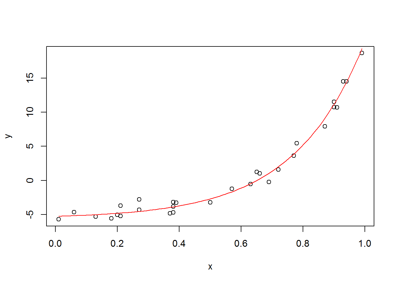
cat(x, sep=', ')## 0.9, 0.27, 0.37, 0.57, 0.91, 0.2, 0.9, 0.94, 0.66, 0.63, 0.06, 0.21, 0.18, 0.69, 0.38, 0.77, 0.5, 0.72, 0.99, 0.38, 0.78, 0.93, 0.21, 0.65, 0.13, 0.27, 0.39, 0.01, 0.38, 0.87cat(y, sep=', ')## 10.77, -4.3, -4.86, -1.23, 10.7, -5.05, 11.56, 14.55, 1.04, -0.54, -4.68, -3.71, -5.58, -0.22, -3.85, 3.64, -3.25, 1.57, 18.69, -3.17, 5.45, 14.55, -5.22, 1.23, -5.31, -2.79, -3.26, -5.72, -4.73, 7.94The only change to the script above is that I need to change the input data as below. I’ll also change the number of iterations by a factor of ten to make sure that isn’t a problem.
import os
os.environ['TF_CPP_MIN_LOG_LEVEL']='2'
import numpy as np
import tensorflow as tf

# Model parameters
a = tf.Variable([.3], dtype=tf.float32)
b = tf.Variable([-.3], dtype=tf.float32)
c = tf.Variable([-.3], dtype=tf.float32)
# Model input and output
x = tf.placeholder(tf.float32)
exp_model = a * tf.exp(c * x) + b
y = tf.placeholder(tf.float32)
# loss
loss = tf.reduce_mean(tf.square(exp_model - y)) # sum of the squares
# optimizer
optimizer = tf.train.GradientDescentOptimizer(0.01)
train = optimizer.minimize(loss)
# training data
# x_train = [1,2,3,4]
# y_train = [0,-1,-2,-3]
# NEW DATA
x_train = [0.9, 0.27, 0.37, 0.57, 0.91, 0.2, 0.9, 0.94, 0.66, 0.63, 0.06, 0.21, 0.18, 0.69, 0.38, 0.77, 0.5, 0.72, 0.99, 0.38, 0.78, 0.93, 0.21, 0.65, 0.13, 0.27, 0.39, 0.01, 0.38, 0.87]
y_train = [10.77, -4.3, -4.86, -1.23, 10.7, -5.05, 11.56, 14.55, 1.04, -0.54, -4.68, -3.71, -5.58, -0.22, -3.85, 3.64, -3.25, 1.57, 18.69, -3.17, 5.45, 14.55, -5.22, 1.23, -5.31, -2.79, -3.26, -5.72, -4.73, 7.94]

# training loop
init = tf.global_variables_initializer()
sess = tf.Session()
sess.run(init) # reset values to wrong
for i in range(10000):
  sess.run(train, {x:x_train, y:y_train})

# evaluate training accuracy
curr_a, curr_b, curr_c, curr_loss = sess.run([a, b, c, loss], {x:x_train, y:y_train})
print("a: %s \nb: %s \nc: %s \nloss: %s"%(curr_a, curr_b, curr_c, curr_loss))
## a: [-32.52795029]
## b: [ 21.62292099]
## c: [-1.09328878]
## loss: 16.1457The values it outputs, shown below, are nowhere near the input values.
plot(x, y)
a <- -32.52795029
b <- 21.62292099
c <- -1.09328878
curve(a*exp(c*x) + b, add=T, col=2)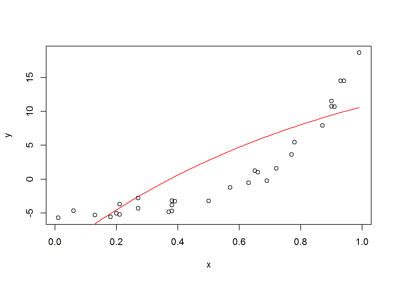
And the plot shows that it looks terrible. I tried restarting it with different starting values and it was still horrible.
Noiseless exponential data
Let me try again but with no noise in the data.
y_nonoise <- round(a*exp(c*x) + b + rnorm(n, 0, 1), 2)
cat(y_nonoise, sep=', ')## 8.4, -4.15, 1.07, 5.01, 9.37, -4.25, 9.09, 12.42, 5.02, 5.23, -8.59, -3.61, -5.27, 4.1, -1.11, 7.96, 2.78, 5.88, 10.49, -0.66, 8, 8.43, -3.87, 5.89, -6.53, -2.57, 0.64, -11.2, 0.03, 9.72The full code is below, I reduced the number of iterations back to the original value.
import os
os.environ['TF_CPP_MIN_LOG_LEVEL']='2'
import numpy as np
import tensorflow as tf
# Model parameters
a = tf.Variable([.0], dtype=tf.float32)
b = tf.Variable([-.0], dtype=tf.float32)
c = tf.Variable([.0], dtype=tf.float32)
# Model input and output
x = tf.placeholder(tf.float32)
exp_model = a * tf.exp(c * x) + b
y = tf.placeholder(tf.float32)
# loss
loss = tf.reduce_mean(tf.square(exp_model - y)) # sum of the squares
# optimizer
optimizer = tf.train.GradientDescentOptimizer(0.01)
train = optimizer.minimize(loss)
# training data
# NEW DATA NO NOISE
x_train = [0.9, 0.27, 0.37, 0.57, 0.91, 0.2, 0.9, 0.94, 0.66, 0.63, 0.06, 0.21, 0.18, 0.69, 0.38, 0.77, 0.5, 0.72, 0.99, 0.38, 0.78, 0.93, 0.21, 0.65, 0.13, 0.27, 0.39, 0.01, 0.38, 0.87]
y_train = [10.12, -6.11, -2.81, -0.84, 11.71, -4.56, 10.81, 16.86, -0.56, -0.54, -4.93, -4.18, -5.07, -1.16, -5.16, 4.23, -2.72, 1.06, 19.23, -4.71, 4.54, 12.13, -4.43, 0.24, -4.97, -4.53, -3.56, -5.91, -4.02, 9.77]
# training loop
init = tf.global_variables_initializer()
sess = tf.Session()
sess.run(init) # reset values to wrong
for i in range(1000):
sess.run(train, {x:x_train, y:y_train})
# evaluate training accuracy
curr_a, curr_b, curr_c, curr_loss = sess.run([a, b, c, loss], {x:x_train, y:y_train})
print("a: %s \nb: %s \nc: %s \nloss: %s"%(curr_a, curr_b, curr_c, curr_loss))
## a: [-13.35965538]
## b: [ 6.38554287]
## c: [-1.93131614]
## loss: 27.3156The output is still awful. No clue why this is happening.
Change of parameters
Let me try one more time, but with no randomness, \(c\) more negative, and \(a\) and \(b\) smaller.
set.seed(0)
a <- 1.32
b <- -0.6
c <- -4.4
n <- 30
x <- round(runif(30), 2)
y <- round(a*exp(c*x) + b , 2)
plot(x, y)
curve(a*exp(c*x) + b, add=T, col=2)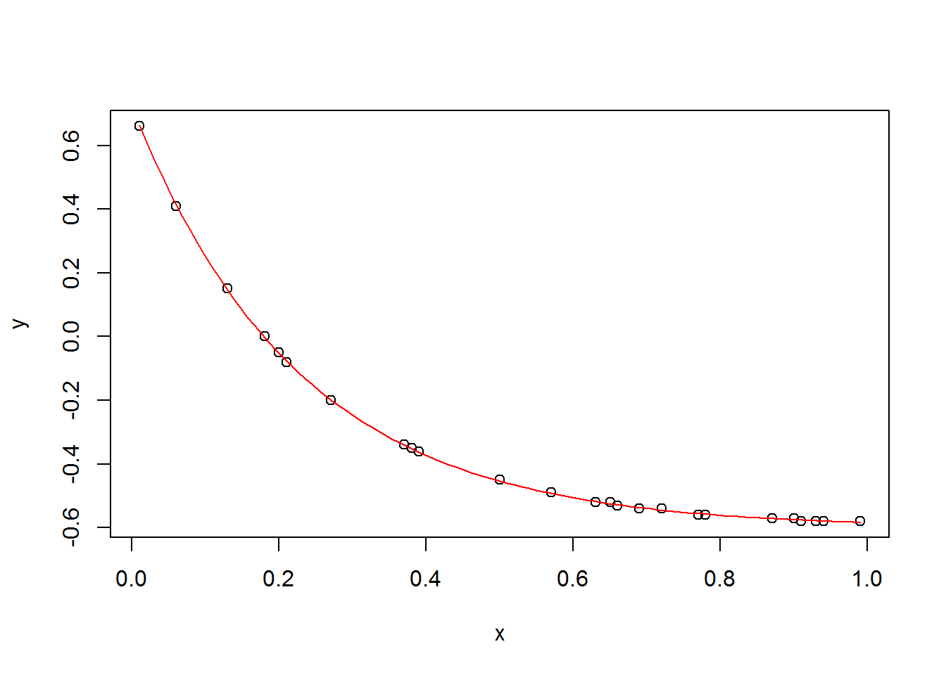
cat(y, sep=', ')## -0.57, -0.2, -0.34, -0.49, -0.58, -0.05, -0.57, -0.58, -0.53, -0.52, 0.41, -0.08, 0, -0.54, -0.35, -0.56, -0.45, -0.54, -0.58, -0.35, -0.56, -0.58, -0.08, -0.52, 0.15, -0.2, -0.36, 0.66, -0.35, -0.57import os
os.environ['TF_CPP_MIN_LOG_LEVEL']='2'
import numpy as np
import tensorflow as tf
# Model parameters
a = tf.Variable([.0], dtype=tf.float32)
b = tf.Variable([-.0], dtype=tf.float32)
c = tf.Variable([.0], dtype=tf.float32)
# Model input and output
x = tf.placeholder(tf.float32)
exp_model = a * tf.exp(c * x) + b
y = tf.placeholder(tf.float32)
# loss
loss = tf.reduce_mean(tf.square(exp_model - y)) # sum of the squares
# optimizer
optimizer = tf.train.GradientDescentOptimizer(0.01)
train = optimizer.minimize(loss)
# training data
x_train = [0.9, 0.27, 0.37, 0.57, 0.91, 0.2, 0.9, 0.94, 0.66, 0.63, 0.06, 0.21, 0.18, 0.69, 0.38, 0.77, 0.5, 0.72, 0.99, 0.38, 0.78, 0.93, 0.21, 0.65, 0.13, 0.27, 0.39, 0.01, 0.38, 0.87]
y_train = [-0.57, -0.2, -0.34, -0.49, -0.58, -0.05, -0.57, -0.58, -0.53, -0.52, 0.41, -0.08, 0, -0.54, -0.35, -0.56, -0.45, -0.54, -0.58, -0.35, -0.56, -0.58, -0.08, -0.52, 0.15, -0.2, -0.36, 0.66, -0.35, -0.57]
# training loop
init = tf.global_variables_initializer()
sess = tf.Session()
sess.run(init) # reset values to wrong
for i in range(1000):
sess.run(train, {x:x_train, y:y_train})
# evaluate training accuracy
curr_a, curr_b, curr_c, curr_loss = sess.run([a, b, c, loss], {x:x_train, y:y_train})
print("a: %s \nb: %s \nc: %s \nloss: %s"%(curr_a, curr_b, curr_c, curr_loss))## a: [-0.26286733]
## b: [-0.0292428]
## c: [ 0.33243284]
## loss: 0.08065These results are a little less egregious.
This curve does not look that good. I’m giving up for today.
plot(x, y)
a <- -0.26286733
b <- -0.0292428
c <- 0.33243284
curve(a*exp(c*x) + b, add=T, col=2)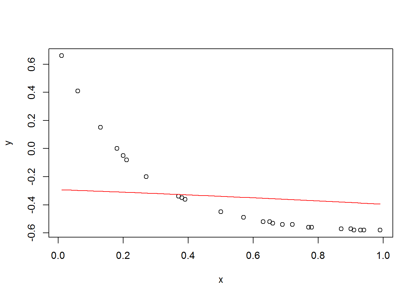
Better starting values
What if I start if with near correct values? We don’t want it to be too sensitive to initial values, but if this doesn’t work then it is hopeless.
import os
os.environ['TF_CPP_MIN_LOG_LEVEL']='2'
import numpy as np
import tensorflow as tf
# Model parameters
a = tf.Variable([1.3], dtype=tf.float32)
b = tf.Variable([-.59], dtype=tf.float32)
c = tf.Variable([-4.3], dtype=tf.float32)
# Model input and output
x = tf.placeholder(tf.float32)
exp_model = a * tf.exp(c * x) + b
y = tf.placeholder(tf.float32)
# loss
loss = tf.reduce_mean(tf.square(exp_model - y)) # sum of the squares
# optimizer
optimizer = tf.train.GradientDescentOptimizer(0.01)
train = optimizer.minimize(loss)
# training data
x_train = [0.9, 0.27, 0.37, 0.57, 0.91, 0.2, 0.9, 0.94, 0.66, 0.63, 0.06, 0.21, 0.18, 0.69, 0.38, 0.77, 0.5, 0.72, 0.99, 0.38, 0.78, 0.93, 0.21, 0.65, 0.13, 0.27, 0.39, 0.01, 0.38, 0.87]
y_train = [-0.57, -0.2, -0.34, -0.49, -0.58, -0.05, -0.57, -0.58, -0.53, -0.52, 0.41, -0.08, 0, -0.54, -0.35, -0.56, -0.45, -0.54, -0.58, -0.35, -0.56, -0.58, -0.08, -0.52, 0.15, -0.2, -0.36, 0.66, -0.35, -0.57]
# training loop
init = tf.global_variables_initializer()
sess = tf.Session()
sess.run(init) # reset values to wrong
for i in range(10000):
sess.run(train, {x:x_train, y:y_train})
# evaluate training accuracy
curr_a, curr_b, curr_c, curr_loss = sess.run([a, b, c, loss], {x:x_train, y:y_train})
print("a: %s \nb: %s \nc: %s \nloss: %s"%(curr_a, curr_b, curr_c, curr_loss))
## a: [ 1.31232285]
## b: [-0.60362089]
## c: [-4.31497335]
## loss: 1.4961e-05This gives values close to the truth.
How about a little further away?
import os
os.environ['TF_CPP_MIN_LOG_LEVEL']='2'
import numpy as np
import tensorflow as tf
# Model parameters
a = tf.Variable([1.6], dtype=tf.float32)
b = tf.Variable([-.9], dtype=tf.float32)
c = tf.Variable([-3.6], dtype=tf.float32)
# Model input and output
x = tf.placeholder(tf.float32)
exp_model = a * tf.exp(c * x) + b
y = tf.placeholder(tf.float32)
# loss
loss = tf.reduce_mean(tf.square(exp_model - y)) # sum of the squares
# optimizer
optimizer = tf.train.GradientDescentOptimizer(0.01)
train = optimizer.minimize(loss)
# training data
x_train = [0.9, 0.27, 0.37, 0.57, 0.91, 0.2, 0.9, 0.94, 0.66, 0.63, 0.06, 0.21, 0.18, 0.69, 0.38, 0.77, 0.5, 0.72, 0.99, 0.38, 0.78, 0.93, 0.21, 0.65, 0.13, 0.27, 0.39, 0.01, 0.38, 0.87]
y_train = [-0.57, -0.2, -0.34, -0.49, -0.58, -0.05, -0.57, -0.58, -0.53, -0.52, 0.41, -0.08, 0, -0.54, -0.35, -0.56, -0.45, -0.54, -0.58, -0.35, -0.56, -0.58, -0.08, -0.52, 0.15, -0.2, -0.36, 0.66, -0.35, -0.57]
# training loop
init = tf.global_variables_initializer()
sess = tf.Session()
sess.run(init) # reset values to wrong
for i in range(10000):
sess.run(train, {x:x_train, y:y_train})
# evaluate training accuracy
curr_a, curr_b, curr_c, curr_loss = sess.run([a, b, c, loss], {x:x_train, y:y_train})
print("a: %s \nb: %s \nc: %s \nloss: %s"%(curr_a, curr_b, curr_c, curr_loss))
## a: [ 1.2807374]
## b: [-0.63670284]
## c: [-3.75594163]
## loss: 0.000446578This gives nearly the same results are before, which is a good sign.
Solving the problem
After spending the day using TensorFlow and getting used to it, I figured out what was probably causing the problem. It wasn’t the data or any part of the model coding. Rather it has to do with the parameter optimization.
I should have tried different step sizes, and maybe more iterations if the step size was made too small.
Let me return to the noisy data. I will reduce the step size to 0.001, whereas I had been using 0.01 up until now.
import os
os.environ['TF_CPP_MIN_LOG_LEVEL']='2'
import numpy as np
import tensorflow as tf
# Model parameters
a = tf.Variable([.3], dtype=tf.float32)
b = tf.Variable([-.3], dtype=tf.float32)
c = tf.Variable([-.3], dtype=tf.float32)
# Model input and output
x = tf.placeholder(tf.float32)
exp_model = a * tf.exp(c * x) + b
y = tf.placeholder(tf.float32)
# loss
loss = tf.reduce_mean(tf.square(exp_model - y)) # sum of the squares
# optimizer
optimizer = tf.train.GradientDescentOptimizer(0.001)
train = optimizer.minimize(loss)
# training data
# x_train = [1,2,3,4]
# y_train = [0,-1,-2,-3]
# NEW DATA
x_train = [0.9, 0.27, 0.37, 0.57, 0.91, 0.2, 0.9, 0.94, 0.66, 0.63, 0.06, 0.21, 0.18, 0.69, 0.38, 0.77, 0.5, 0.72, 0.99, 0.38, 0.78, 0.93, 0.21, 0.65, 0.13, 0.27, 0.39, 0.01, 0.38, 0.87]
y_train = [10.77, -4.3, -4.86, -1.23, 10.7, -5.05, 11.56, 14.55, 1.04, -0.54, -4.68, -3.71, -5.58, -0.22, -3.85, 3.64, -3.25, 1.57, 18.69, -3.17, 5.45, 14.55, -5.22, 1.23, -5.31, -2.79, -3.26, -5.72, -4.73, 7.94]
# training loop
init = tf.global_variables_initializer()
sess = tf.Session()
sess.run(init) # reset values to wrong
for i in range(10000):
sess.run(train, {x:x_train, y:y_train})
# evaluate training accuracy
curr_a, curr_b, curr_c, curr_loss = sess.run([a, b, c, loss], {x:x_train, y:y_train})
print("a: %s \nb: %s \nc: %s \nloss: %s"%(curr_a, curr_b, curr_c, curr_loss))## a: [ 0.33135614]
## b: [-5.52935982]
## c: [ 4.34632301]
## loss: 0.598727x <- c(0.9, 0.27, 0.37, 0.57, 0.91, 0.2, 0.9, 0.94, 0.66, 0.63, 0.06, 0.21, 0.18, 0.69, 0.38, 0.77, 0.5, 0.72, 0.99, 0.38, 0.78, 0.93, 0.21, 0.65, 0.13, 0.27, 0.39, 0.01, 0.38, 0.87)
y <- c(10.77, -4.3, -4.86, -1.23, 10.7, -5.05, 11.56, 14.55, 1.04, -0.54, -4.68, -3.71, -5.58, -0.22, -3.85, 3.64, -3.25, 1.57, 18.69, -3.17, 5.45, 14.55, -5.22, 1.23, -5.31, -2.79, -3.26, -5.72, -4.73, 7.94)
a <- 0.33135614
b <- -5.52935982
c <- 4.34632301
plot(x, y)
curve(a*exp(c*x)+b, add=T, col=2)
We can see that it is a perfect fit. The whole time that I thought there was a problem, it was just a parameter selection issue.
How I should have seen this problem earlier
If I had printed the loss after each iteration, I probably would have seen something fishy. It probably would jump around a lot since the step size was too big, or else it would still be in the process of decreasing and need more time to converge. Let me try the original model again with the big step size 0.01 and print out the loss after each iteration.
import os
os.environ['TF_CPP_MIN_LOG_LEVEL']='2'
import numpy as np
import tensorflow as tf
# Model parameters
a = tf.Variable([.3], dtype=tf.float32)
b = tf.Variable([-.3], dtype=tf.float32)
c = tf.Variable([-.3], dtype=tf.float32)
# Model input and output
x = tf.placeholder(tf.float32)
exp_model = a * tf.exp(c * x) + b
y = tf.placeholder(tf.float32)
# loss
loss = tf.reduce_mean(tf.square(exp_model - y)) # sum of the squares
# optimizer
optimizer = tf.train.GradientDescentOptimizer(0.01)
train = optimizer.minimize(loss)
# training data
# x_train = [1,2,3,4]
# y_train = [0,-1,-2,-3]
# NEW DATA
x_train = [0.9, 0.27, 0.37, 0.57, 0.91, 0.2, 0.9, 0.94, 0.66, 0.63, 0.06, 0.21, 0.18, 0.69, 0.38, 0.77, 0.5, 0.72, 0.99, 0.38, 0.78, 0.93, 0.21, 0.65, 0.13, 0.27, 0.39, 0.01, 0.38, 0.87]
y_train = [10.77, -4.3, -4.86, -1.23, 10.7, -5.05, 11.56, 14.55, 1.04, -0.54, -4.68, -3.71, -5.58, -0.22, -3.85, 3.64, -3.25, 1.57, 18.69, -3.17, 5.45, 14.55, -5.22, 1.23, -5.31, -2.79, -3.26, -5.72, -4.73, 7.94]
# training loop
init = tf.global_variables_initializer()
sess = tf.Session()
sess.run(init) # reset values to wrong
for i in range(10000):
if i%500 == 0:
loss_i = sess.run(loss, {x:x_train, y:y_train})
print("Iter %d:\tLoss: %.3f"%(i, loss_i))
sess.run(train, {x:x_train, y:y_train})
# evaluate training accuracy
curr_a, curr_b, curr_c, curr_loss = sess.run([a, b, c, loss], {x:x_train, y:y_train})
print("a: %s \nb: %s \nc: %s \nloss: %s"%(curr_a, curr_b, curr_c, curr_loss))## Iter 0: Loss: 52.006
## Iter 500: Loss: 29.149
## Iter 1000: Loss: 22.839
## Iter 1500: Loss: 19.896
## Iter 2000: Loss: 18.262
## Iter 2500: Loss: 17.230
## Iter 3000: Loss: 16.515
## Iter 3500: Loss: 15.986
## Iter 4000: Loss: 15.575
## Iter 4500: Loss: 15.245
## Iter 5000: Loss: 14.971
## Iter 5500: Loss: 14.740
## Iter 6000: Loss: 14.542
## Iter 6500: Loss: 14.368
## Iter 7000: Loss: 14.215
## Iter 7500: Loss: 14.079
## Iter 8000: Loss: 13.956
## Iter 8500: Loss: 15.746
## Iter 9000: Loss: 15.996
## Iter 9500: Loss: 16.102
## a: [-32.52795029]
## b: [ 21.62292099]
## c: [-1.09328878]
## loss: 16.1457It looks like the loss decreased for the first 8,000 iterations, then started increasing again. More iterations might not have helped since it looks like it started to diverge. Divergence is a sign that a smaller step size is needed.